The Basics#
PyAutoFit is a Python based probabilistic programming language for model fitting and Bayesian inference of large datasets.
The basic PyAutoFit API allows us a user to quickly compose a probabilistic model and fit it to data via a log likelihood function, using a range of non-linear search algorithms (e.g. MCMC, nested sampling).
This overview gives a run through of:
Models: Use Python classes to compose the model which is fitted to data.
Instances: Create instances of the model via its Python class.
Analysis: Define an
Analysisclass which includes the log likelihood function that fits the model to the data.Searches: Choose an MCMC, nested sampling or maximum likelihood estimator non-linear search algorithm that fits the model to the data.
Model Fit: Fit the model to the data using the chosen non-linear search, with on-the-fly results and visualization.
Results: Use the results of the search to interpret and visualize the model fit.
Samples: Use the samples of the search to inspect the parameter samples and visualize the probability density function of the results.
Multiple Datasets: Dedicated support for simultaneously fitting multiple datasets, enabling scalable analysis of large datasets.
This overviews provides a high level of the basic API, with more advanced functionality described in the following overviews and the PyAutoFit cookbooks.
Example#
To illustrate PyAutoFit we’ll use the example modeling problem of fitting a 1D Gaussian profile to noisy data.
To begin, lets import autofit (and numpy) using the convention below:
import autofit as af
import numpy as np
The example data with errors (black) is shown below:
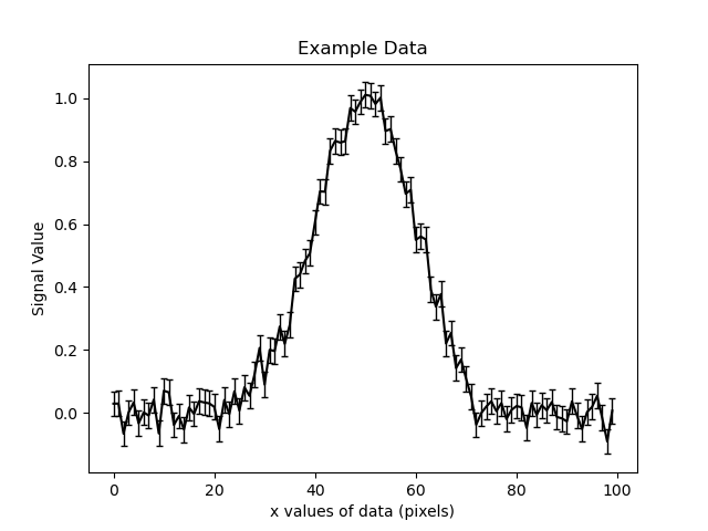
The 1D signal was generated using a 1D Gaussian profile of the form:
Where:
x: The x-axis coordinate where theGaussianis evaluated.
N: The overall normalization of the Gaussian.
sigma: Describes the size of the Gaussian.
Our modeling task is to fit the data with a 1D Gaussian and recover its parameters (x, N, sigma).
Model#
We therefore need to define a 1D Gaussian as a PyAutoFit model.
We do this by writing it as the following Python class:
class Gaussian:
    def __init__(
        self,
        centre=0.0,  # <- PyAutoFit recognises these constructor arguments
        normalization=0.1,  # <- are the Gaussian`s model parameters.
        sigma=0.01,
    ):
        """
        Represents a 1D `Gaussian` profile, which can be treated as a
        PyAutoFit model-component whose free parameters (centre,
        normalization and sigma) are fitted for by a non-linear search.

        Parameters
        ----------
        centre
            The x coordinate of the profile centre.
        normalization
            Overall normalization of the `Gaussian` profile.
        sigma
            The sigma value controlling the size of the Gaussian.
        """
        self.centre = centre
        self.normalization = normalization
        self.sigma = sigma

    def model_data_from(self, xvalues: np.ndarray) -> np.ndarray:
        """
        Returns the 1D Gaussian profile on a line of Cartesian x coordinates.

        The input xvalues are translated to a coordinate system centred on the
        Gaussian, by subtracting its centre.

        The output is referred to as the `model_data` to signify that it is
        a representation of the data from the model.

        Parameters
        ----------
        xvalues
            The x coordinates for which the Gaussian is evaluated.
        """
        transformed_xvalues = xvalues - self.centre

        return np.multiply(
            np.divide(self.normalization, self.sigma * np.sqrt(2.0 * np.pi)),
            np.exp(-0.5 * np.square(np.divide(transformed_xvalues, self.sigma))),
        )
The PyAutoFit model above uses the following format:
The name of the class is the name of the model, in this case, “Gaussian”.
The input arguments of the constructor (the
__init__method) are the parameters of the model, in this casecentre,normalizationandsigma.The default values of the input arguments define whether a parameter is a single-valued
floator a multi-valuedtuple. In this case, all 3 input parameters are floats.It includes functions associated with that model component, which are used when fitting the model to data.
To compose a model using the Gaussian class above we use the af.Model object.
model = af.Model(Gaussian)
print("Model ``Gaussian`` object: \n")
print(model)
This gives the following output:
Model `Gaussian` object:

Gaussian (centre, UniformPrior [1], lower_limit = 0.0, upper_limit = 100.0),
(normalization, LogUniformPrior [2], lower_limit = 1e-06, upper_limit = 1000000.0),
(sigma, UniformPrior [3], lower_limit = 0.0, upper_limit = 25.0)
Note
PyAutoFit supports the use of configuration files defining the default priors on every model parameter, which is how the priors above were set. This allows the user to set up default priors in a consistent and concise way, but with a high level of customization and extensibility. The use of config files to set up default behaviour is described in the configs cookbook.
The model has a total of 3 parameters:
print(model.total_free_parameters)
All model information is given by printing its info attribute:
print(model.info)
This gives the following output:
Total Free Parameters = 3

model                         Gaussian (N=3)

centre                        UniformPrior [1], lower_limit = 0.0, upper_limit = 100.0
normalization                 LogUniformPrior [2], lower_limit = 1e-06, upper_limit = 1000000.0
sigma                         UniformPrior [3], lower_limit = 0.0, upper_limit = 25.0
The priors can be manually altered as follows:
model.centre = af.UniformPrior(lower_limit=0.0, upper_limit=100.0)
model.normalization = af.UniformPrior(lower_limit=0.0, upper_limit=1e2)
model.sigma = af.UniformPrior(lower_limit=0.0, upper_limit=30.0)
Printing the model.info displayed these updated priors.
print(model.info)
This gives the following output:
Total Free Parameters = 3

model                                   Gaussian (N=3)

centre                                  UniformPrior [4], lower_limit = 0.0, upper_limit = 100.0
normalization                           UniformPrior [5], lower_limit = 0.0, upper_limit = 100.0
sigma                                   UniformPrior [6], lower_limit = 0.0, upper_limit = 30.0
Note
The example above uses the most basic PyAutoFit API to compose a simple model. The API is highly extensible and can scale to models with thousands of parameters, complex hierarchies and relationships between parameters. A complete overview is given in the model cookbook.
Instances#
Instances of a PyAutoFit model (created via af.Model) can be generated by mapping an input vector of parameter
values to create an instance of the model’s Python class.
To define the input vector correctly, we need to know the order of parameters in the model. This information is
contained in the model’s paths attribute.
print(model.paths)
This gives the following output:
[('centre',), ('normalization',), ('sigma',)]
We input values for the three free parameters of our model in the order specified by the paths
attribute (i.e., centre=30.0, normalization=2.0, and sigma=3.0):
instance = model.instance_from_vector(vector=[30.0, 2.0, 3.0])
This is an instance of the Gaussian class.
print("Model Instance: \n")
print(instance)
This gives the following output:
Model Instance:

<__main__.Gaussian object at 0x7f3e37cb1990>
It has the parameters of the Gaussian with the values input above.
print("Instance Parameters \n")
print("x = ", instance.centre)
print("normalization = ", instance.normalization)
print("sigma = ", instance.sigma)
This gives the following output:
Instance Parameters

x =  30.0
normalization =  2.0
sigma =  3.0
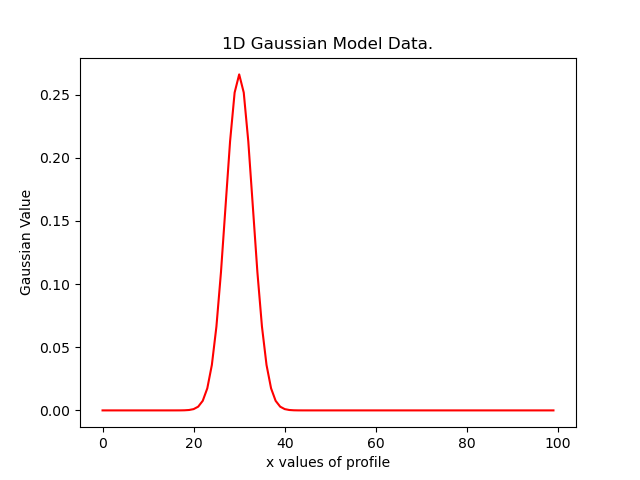
We can use functions associated with the class, specifically the model_data_from function, to
create a realization of the Gaussian and plot it.
xvalues = np.arange(0.0, 100.0, 1.0)

model_data = instance.model_data_from(xvalues=xvalues)

plt.plot(xvalues, model_data, color="r")
plt.title("1D Gaussian Model Data.")
plt.xlabel("x values of profile")
plt.ylabel("Gaussian Value")
plt.show()
plt.clf()
Here is what the plot looks like:
Note
Mapping models to instance of their Python classes is an integral part of the core PyAutoFit API. It enables the advanced model composition and results management tools illustrated in the following overviews and cookbooks.
Analysis#
We now tell PyAutoFit how to fit the model to the data.
We define an Analysis class, which includes:
An
__init__constructor that takesdataandnoise_mapas inputs (this can be extended with additional elements necessary for fitting the model to the data).A
log_likelihood_functionthat defines how to fit aninstanceof the model to the data and return a log likelihood value.
Read the comments and docstrings of the Analysis class in detail for a full description of how the analysis works.
class Analysis(af.Analysis):
    def __init__(self, data: np.ndarray, noise_map: np.ndarray):
        """
        The ``Analysis`` class acts as an interface between the data and
        model in **PyAutoFit**.

        Its ``log_likelihood_function`` defines how the model is fitted to
        the data and it is called many times by the non-linear search fitting
        algorithm.

        In this example the ``Analysis`` ``__init__`` constructor only contains
        the ``data`` and ``noise-map``, but it can be easily extended to
        include other quantities.

        Parameters
        ----------
        data
            A 1D numpy array containing the data (e.g. a noisy 1D signal)
            fitted in the readthedocs and workspace examples.
        noise_map
            A 1D numpy array containing the noise values of the data, used
            for computing the goodness of fit metric, the log likelihood.
        """

        super().__init__()

        self.data = data
        self.noise_map = noise_map

    def log_likelihood_function(self, instance) -> float:
        """
        Returns the log likelihood of a fit of a 1D Gaussian to the dataset.

        The data is fitted using an ``instance`` of the ``Gaussian`` class
        where its ``model_data_from`` is called in order to
        create a model data representation of the Gaussian that is fitted to the data.
        """

        """
        The ``instance`` that comes into this method is an instance of the ``Gaussian``
        model above, which was created via ``af.Model()``.

        The parameter values are chosen by the non-linear search and therefore are based
        on where it has mapped out the high likelihood regions of parameter space are.

        The lines of Python code are commented out below to prevent excessive print
        statements when we run the non-linear search, but feel free to uncomment
        them and run the search to see the parameters of every instance
        that it fits.

        # print("Gaussian Instance:")
        # print("Centre = ", instance.centre)
        # print("Normalization = ", instance.normalization)
        # print("Sigma = ", instance.sigma)
        """

        """
        Get the range of x-values the data is defined on, to evaluate the model of the Gaussian.
        """
        xvalues = np.arange(self.data.shape[0])

        """
        Use these xvalues to create model data of our Gaussian.
        """
        model_data = instance.model_data_from(xvalues=xvalues)

        """
        Fit the model gaussian line data to the observed data, computing the residuals,
        chi-squared and log likelihood.
        """
        residual_map = self.data - model_data
        chi_squared_map = (residual_map / self.noise_map) ** 2.0
        chi_squared = sum(chi_squared_map)
        noise_normalization = np.sum(np.log(2 * np.pi * self.noise_map**2.0))
        log_likelihood = -0.5 * (chi_squared + noise_normalization)

        return log_likelihood
Create an instance of the Analysis class by passing the data and noise_map.
analysis = Analysis(data=data, noise_map=noise_map)
Note
The Analysis class shown above is the simplest example possible. The API is highly extensible and can include
model-specific output, visualization and latent variable calculations. A complete overview is given in the
analysis cookbook.
Non Linear Search#
We now have a model ready to fit the data and an analysis class that performs this fit.
Next, we need to select a fitting algorithm, known as a “non-linear search,” to fit the model to the data.
PyAutoFit supports various non-linear searches, which can be broadly categorized into three types: MCMC (Markov Chain Monte Carlo), nested sampling, and maximum likelihood estimators.
For this example, we will use the nested sampling algorithm called Dynesty.
search = af.DynestyStatic(
    nlive=100, # Example how to customize the search settings
)
The default settings of the non-linear search are specified in the configuration files of PyAutoFit, just like the default priors of the model components above. The ensures the basic API of your code is concise and readable, but with the flexibility to customize the search to your specific model-fitting problem.
Note
PyAutoFit supports a wide range of non-linear searches, including detailed visualuzation, support for parallel processing, and GPU and gradient based methods using the library JAX (https://jax.readthedocs.io/en/latest/). A complete overview is given in the searches cookbook.
Model Fit#
We begin the non-linear search by passing the model and analysis to its fit method.
print(
    The non-linear search has begun running.
    This Jupyter notebook cell with progress once the search
    has completed - this could take a few minutes!
)

result = search.fit(model=model, analysis=analysis)

print("The search has finished run - you may now continue the notebook.")
Result#
The result object returned by the fit provides information on the results of the non-linear search.
The info attribute shows the result in a readable format.
print(result.info)
The output is as follows:
Bayesian Evidence                       167.54413502
Maximum Log Likelihood                  183.29775793
Maximum Log Posterior                   183.29775793

model                                   Gaussian (N=3)

Maximum Log Likelihood Model:

centre                                  49.880
normalization                           24.802
sigma                                   9.849


Summary (3.0 sigma limits):

centre                                  49.88 (49.51, 50.29)
normalization                           24.80 (23.98, 25.67)
sigma                                   9.84 (9.47, 10.25)


Summary (1.0 sigma limits):

centre                                  49.88 (49.75, 50.01)
normalization                           24.80 (24.54, 25.11)
sigma                                   9.84 (9.73, 9.97)
Results are returned as instances of the model, as illustrated above in the instance section.
For example, we can print the result’s maximum likelihood instance.
print(result.max_log_likelihood_instance)

print("\nModel-fit Max Log-likelihood Parameter Estimates: \n")
print("Centre = ", result.max_log_likelihood_instance.centre)
print("Normalization = ", result.max_log_likelihood_instance.normalization)
print("Sigma = ", result.max_log_likelihood_instance.sigma)
This gives the following output:
Model-fit Max Log-likelihood Parameter Estimates:

Centre =  49.87954357347897
Normalization =  24.80227227310798
Sigma =  9.84888033338011
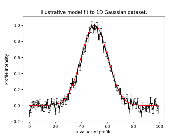
A benefit of the result being an instance is that we can use any of its methods to inspect the results.
Below, we use the maximum likelihood instance to compare the maximum likelihood Gaussian to the data.
model_data = result.max_log_likelihood_instance.model_data_from(
    xvalues=np.arange(data.shape[0])
)

plt.errorbar(
    x=xvalues, y=data, yerr=noise_map, color="k", ecolor="k", elinewidth=1, capsize=2
)
plt.plot(xvalues, model_data, color="r")
plt.title("Dynesty model fit to 1D Gaussian dataset.")
plt.xlabel("x values of profile")
plt.ylabel("Profile normalization")
plt.show()
plt.close()
The plot appears as follows:
Note
Result objects contain a wealth of information on the model-fit, including parameter and error estimates. They can be extensively customized to include additional information specific to your scientific problem. A complete overview is given in the results cookbook.
Samples#
The results object also contains a Samples object, which contains all information on the non-linear search.
This includes parameter samples, log likelihood values, posterior information and results internal to the specific algorithm (e.g. the internal dynesty samples).
Below we use the samples to plot the probability density function cornerplot of the results.
plotter = aplt.NestPlotter(samples=result.samples)
plotter.corner_anesthetic()
The plot appears as follows:

Note
The results cookbook also provides a run through of the samples object API.
Multiple Datasets#
Many model-fitting problems require multiple datasets to be fitted simultaneously in order to provide the best constraints on the model.
In PyAutoFit, all you have to do to fit multiple datasets is combine them with the model via AnalysisFactor
objects.
analysis_0 = Analysis(data=data, noise_map=noise_map)
analysis_1 = Analysis(data=data, noise_map=noise_map)

analysis_list = [analysis_0, analysis_1]

analysis_factor_list = []

for analysis in analysis_list:

    # The model can be customized here so that different model parameters are tied to each analysis.
    model_analysis = model.copy()

    analysis_factor = af.AnalysisFactor(prior_model=model_analysis, analysis=analysis)

    analysis_factor_list.append(analysis_factor)
All AnalysisFactor objects are combined into a FactorGraphModel, which represents a global model fit to
multiple datasets using a graphical model structure.
The key outcomes of this setup are:
The individual log likelihoods from each
Analysisobject are summed to form the total log likelihood evaluated during the model-fitting process.Results from all datasets are output to a unified directory, with subdirectories for visualizations from each analysis object, as defined by their
visualizemethods.
This is a basic use of PyAutoFit’s graphical modeling capabilities, which support advanced hierarchical and probabilistic modeling for large, multi-dataset analyses.
To inspect the model, we print factor_graph.global_prior_model.info.
print(factor_graph.global_prior_model.info)
To fit multiple datasets, we pass the FactorGraphModel to a non-linear search.
Unlike single-dataset fitting, we now pass the factor_graph.global_prior_model as the model and
the factor_graph itself as the analysis object.
This structure enables simultaneous fitting of multiple datasets in a consistent and scalable way.
search = af.DynestyStatic(
    nlive=100,
)

result_list = search.fit(model=factor_graph.global_prior_model, analysis=factor_graph)
Note
In the simple example above, instances of the same Analysis class (analysis_0 and analysis_1) were
combined. However, different Analysis classes can also be combined. This is useful when fitting different
datasets that each require a unique log_likelihood_function to be fitted simultaneously. For more detailed
information and a dedicated API for customizing how the model changes across different datasets, refer to
the [multiple datasets cookbook](https://pyautofit.readthedocs.io/en/latest/cookbooks/multiple_datasets.html).
Wrap Up#
This overview covers the basic functionality of PyAutoFit using a simple model, dataset, and model-fitting problem, demonstrating the fundamental aspects of its API.
By now, you should have a clear understanding of how to define and compose your own models, fit them to data using a non-linear search, and interpret the results.
The PyAutoFit API introduced here is highly extensible and customizable, making it adaptable to a wide range of model-fitting problems.
The next overview will delve into setting up a scientific workflow with PyAutoFit, utilizing its API to optimize model-fitting efficiency and scalability for large datasets. This approach ensures that detailed scientific interpretation of the results remains feasible and insightful.
Resources#
The autofit_workspace: repository on GitHub provides numerous examples demonstrating more complex model-fitting tasks.
This includes cookbooks, which provide a concise reference guide to the PyAutoFit API for advanced model-fitting:
[Model Cookbook](https://pyautofit.readthedocs.io/en/latest/cookbooks/model.html): Learn how to compose complex models using multiple Python classes, lists, dictionaries, NumPy arrays and customize their parameterization.
[Analysis Cookbook](https://pyautofit.readthedocs.io/en/latest/cookbooks/search.html): Customize the analysis with model-specific output and visualization to gain deeper insights into your model fits.
[Searches Cookbook](https://pyautofit.readthedocs.io/en/latest/cookbooks/analysis.html): Choose from a variety of non-linear searches and customize their behavior. This includes options like outputting results to hard disk and parallelizing the search process.
[Results Cookbook](https://pyautofit.readthedocs.io/en/latest/cookbooks/result.html): Explore the various results available from a fit, such as parameter estimates, error estimates, model comparison metrics, and customizable visualizations.
[Configs Cookbook](https://pyautofit.readthedocs.io/en/latest/cookbooks/configs.html): Customize default settings using configuration files. This allows you to set priors, search settings, visualization preferences, and more.
[Multiple Dataset Cookbook](https://pyautofit.readthedocs.io/en/latest/cookbooks/multiple_datasets.html): Learn how to fit multiple datasets simultaneously by combining their analysis classes so that their log likelihoods are summed.
These cookbooks provide detailed guides and examples to help you leverage the PyAutoFit API effectively for a wide range of model-fitting tasks.