Scientific Workflow#
A scientific workflow comprises the tasks you perform to conduct a scientific study. This includes fitting models to datasets, interpreting the results, and gaining insights into your scientific problem.
Different problems require different scientific workflows, depending on factors such as model complexity, dataset size, and computational run times. For example, some problems involve fitting a single dataset with many models to gain scientific insights, while others involve fitting thousands of datasets with a single model for large-scale studies.
The PyAutoFit API is flexible, customizable, and extensible, enabling users to develop scientific workflows tailored to their specific problems.
This overview covers the key features of PyAutoFit that support the development of effective scientific workflows:
On The Fly: Display results immediately (e.g., in Jupyter notebooks) to provide instant feedback for adapting your workflow.
Hard Disk Output: Output results to hard disk with high customization, allowing quick and detailed inspection of fits to many datasets.
Visualization: Generate model-specific visualizations to create custom plots that streamline result inspection.
Loading Results: Load results from the hard disk to inspect and interpret the outcomes of a model fit.
Result Customization: Customize the returned results to simplify scientific interpretation.
Model Composition: Extensible model composition makes it easy to fit many models with different parameterizations and assumptions.
Searches: Support for various non-linear searches (e.g., nested sampling, MCMC), including gradient based fitting using JAX, to find the right method for your problem.
Configs: Configuration files that set default model, fitting, and visualization behaviors, streamlining model fitting.
Database: Store results in a relational SQLite3 database, enabling efficient management of large modeling results.
Scaling Up: Guidance on scaling up your scientific workflow from small to large datasets.
On The Fly#
Note
The on-the-fly feature described below is not implemented yet, we are working on it currently. The best way to get on-the-fly output is to output to hard-disk, which is described in the next section. This feature is fully implemented and provides on-the-fly output of results to hard-disk.
When a model fit is running, information about the fit is displayed at user-specified intervals.
The frequency of this on-the-fly output is controlled by a search’s iterations_per_full_update parameter, which
specifies how often this information is output. The example code below outputs on-the-fly information every 1000 iterations:
search = af.DynestyStatic(
    iterations_per_full_update=1000
)
In a Jupyter notebook, the default behavior is for this information to appear in the cell being run and to include:
Text displaying the maximum likelihood model inferred so far and related information.
A visual showing how the search has sampled parameter space so far, providing intuition on how the search is performing.
Here is an image of how this looks:

The most valuable on-the-fly output is often specific to the model and dataset you are fitting. For instance, it
might be a matplotlib subplot showing the maximum likelihood model’s fit to the dataset, complete with residuals
and other diagnostic information.
The on-the-fly output can be fully customized by extending the on_the_fly_output method of the Analysis
class being used to fit the model.
The example below shows how this is done for the simple case of fitting a 1D Gaussian profile:
class Analysis(af.Analysis):
    def __init__(self, data: np.ndarray, noise_map: np.ndarray):
        """
        Example Analysis class illustrating how to customize the on-the-fly output of a model-fit.
        """
        super().__init__()

        self.data = data
        self.noise_map = noise_map

    def on_the_fly_output(self, instance):
        """
        During a model-fit, the `on_the_fly_output` method is called throughout the non-linear search.

        The `instance` passed into the method is maximum log likelihood solution obtained by the model-fit so far and it can be
        used to provide on-the-fly output showing how the model-fit is going.
        """
        xvalues = np.arange(analysis.data.shape[0])

        model_data = instance.model_data_from(xvalues=xvalues)

        """
        The visualizer now outputs images of the best-fit results to hard-disk (checkout `visualizer.py`).
        """
        import matplotlib.pyplot as plt

        plt.errorbar(
            x=xvalues,
            y=self.data,
            yerr=self.noise_map,
            color="k",
            ecolor="k",
            elinewidth=1,
            capsize=2,
        )
        plt.plot(xvalues, model_data, color="r")
        plt.title("Maximum Likelihood Fit")
        plt.xlabel("x value of profile")
        plt.ylabel("Profile Normalization")
        plt.show() # By using `plt.show()` the plot will be displayed in the Jupyter notebook.
Here’s how the visuals appear in a Jupyter Notebook:

In the early stages of setting up a scientific workflow, on-the-fly output is invaluable. It provides immediate feedback on how your model fitting is performing, which is often crucial at the beginning of a project when things might not be going well. It also encourages you to prioritize visualizing your fit and diagnosing whether the process is working correctly.
We highly recommend users starting a new model-fitting problem begin by setting up on-the-fly output!
Hard Disk Output#
By default, a non-linear search does not save its results to the hard disk; the results can only be inspected in a Jupyter Notebook or Python script via the returned result.
However, you can enable the output of non-linear search results to the hard disk by specifying the name and/or path_prefix attributes. These attributes determine how files are named and where results are saved on your hard disk.
Benefits of saving results to the hard disk include:
More efficient inspection of results for multiple datasets compared to using a Jupyter Notebook.
Results are saved on-the-fly, allowing you to check the progress of a fit midway.
Additional information about a fit, such as visualizations, can be saved (see below).
Unfinished runs can be resumed from where they left off if they are terminated.
On high-performance supercomputers, results often need to be saved in this manner.
Here’s how to enable the output of results to the hard disk:
search = af.Emcee(
    path_prefix=path.join("folder_0", "folder_1"),
    name="my_search_name"
)
The screenshot below shows the output folder where all output is enabled:
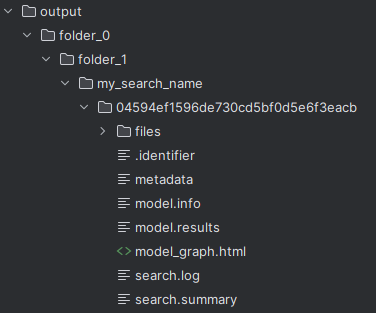
Let’s break down the output folder generated by PyAutoFit:
Unique Identifier: Results are saved in a folder named with a unique identifier composed of random characters. This identifier is automatically generated based on the specific model fit. For scientific workflows involving numerous model fits, this ensures that each fit is uniquely identified without requiring manual updates to output paths.
Info Files: These files contain valuable information about the fit. For instance,
model.infoprovides the complete model composition used in the fit, whilesearch.summarydetails how long the search has been running and other relevant search-specific information.Files Folder: Within the output folder, the
filesdirectory contains detailed information saved as.jsonfiles. For example,model.jsonstores the model configuration used in the fit. This enables researchers to revisit the results later and review how the fit was performed.
PyAutoFit offers extensive tools for customizing hard-disk output. This includes using configuration files to control what information is saved, which helps manage disk space utilization. Additionally, specific .json files tailored to different models can be utilized for more detailed output.
For many scientific workflows, having detailed output for each fit is crucial for thorough inspection and accurate
interpretation of results. However, in scenarios where the volume of output data might overwhelm users or impede
scientific study, this feature can be easily disabled by omitting the name or path prefix when initiating the search.
Visualization#
When search hard-disk output is enabled in PyAutoFit, the visualization of model fits can also be saved directly to disk. This capability is crucial for many scientific workflows as it allows for quick and effective assessment of fit quality.
To accomplish this, you can customize the Visualizer object of an Analysis class with a custom Visualizer class.
This custom class is responsible for generating and saving visual representations of the model fits. By leveraging
this approach, scientists can efficiently visualize and analyze the outcomes of model fitting processes.
class Visualizer(af.Visualizer):

   @staticmethod
   def visualize_before_fit(
       analysis,
       paths: af.DirectoryPaths,
       model: af.AbstractPriorModel
   ):
       """
       Before a model-fit, the `visualize_before_fit` method is called to perform visualization.

       The function receives as input an instance of the `Analysis` class which is being used to perform the fit,
       which is used to perform the visualization (e.g. it contains the data and noise map which are plotted).

       This can output visualization of quantities which do not change during the model-fit, for example the
       data and noise-map.

       The `paths` object contains the path to the folder where the visualization should be output, which is determined
       by the non-linear search `name` and other inputs.
       """

       import matplotlib.pyplot as plt

       xvalues = np.arange(self.data.shape[0])

       plt.errorbar(
           x=xvalues,
           y=analysis.data,
           yerr=analysis.noise_map,
           color="k",
           ecolor="k",
           elinewidth=1,
           capsize=2,
       )
       plt.title("Maximum Likelihood Fit")
       plt.xlabel("x value of profile")
       plt.ylabel("Profile Normalization")
       plt.savefig(path.join(paths.image_path, f"data.png"))
       plt.clf()

   @staticmethod
   def visualize(
       analysis,
       paths: af.DirectoryPaths,
       instance,
       during_analysis
   ):
       """
       During a model-fit, the `visualize` method is called throughout the non-linear search.

       The function receives as input an instance of the `Analysis` class which is being used to perform the fit,
       which is used to perform the visualization (e.g. it generates the model data which is plotted).

       The `instance` passed into the visualize method is maximum log likelihood solution obtained by the model-fit
       so far and it can be used to provide on-the-fly images showing how the model-fit is going.

       The `paths` object contains the path to the folder where the visualization should be output, which is determined
       by the non-linear search `name` and other inputs.
       """
       xvalues = np.arange(analysis.data.shape[0])

       model_data = instance.model_data_from(xvalues=xvalues)
       residual_map = analysis.data - model_data

       """
       The visualizer now outputs images of the best-fit results to hard-disk (checkout `visualizer.py`).
       """
       import matplotlib.pyplot as plt

       plt.errorbar(
           x=xvalues,
           y=analysis.data,
           yerr=analysis.noise_map,
           color="k",
           ecolor="k",
           elinewidth=1,
           capsize=2,
       )
       plt.plot(xvalues, model_data, color="r")
       plt.title("Maximum Likelihood Fit")
       plt.xlabel("x value of profile")
       plt.ylabel("Profile Normalization")
       plt.savefig(path.join(paths.image_path, f"model_fit.png"))
       plt.clf()

       plt.errorbar(
           x=xvalues,
           y=residual_map,
           yerr=analysis.noise_map,
           color="k",
           ecolor="k",
           elinewidth=1,
           capsize=2,
       )
       plt.title("Residuals of Maximum Likelihood Fit")
       plt.xlabel("x value of profile")
       plt.ylabel("Residual")
       plt.savefig(path.join(paths.image_path, f"model_fit.png"))
       plt.clf()
The Analysis class is defined following the same API as before, but now with its Visualizer class attribute
overwritten with the Visualizer class above.
class Analysis(af.Analysis):

    """
    This over-write means the `Visualizer` class is used for visualization throughout the model-fit.

    This `VisualizerExample` object is in the `autofit.example.visualize` module and is used to customize the
    plots output during the model-fit.

    It has been extended with visualize methods that output visuals specific to the fitting of `1D` data.
    """
    Visualizer = Visualizer

    def __init__(self, data, noise_map):
        """
        An Analysis class which illustrates visualization.
        """
        super().__init__()

        self.data = data
        self.noise_map = noise_map

    def log_likelihood_function(self, instance):
        """
        The `log_likelihood_function` is identical to the example above
        """
        xvalues = np.arange(self.data.shape[0])

        model_data = instance.model_data_from(xvalues=xvalues)
        residual_map = self.data - model_data
        chi_squared_map = (residual_map / self.noise_map) ** 2.0
        chi_squared = sum(chi_squared_map)
        noise_normalization = np.sum(np.log(2 * np.pi * noise_map**2.0))
        log_likelihood = -0.5 * (chi_squared + noise_normalization)

        return log_likelihood
Visualization of the results of the non-linear search, for example the “Probability Density Function”, are also automatically output during the model-fit on the fly.
Loading Results#
In your scientific workflow, you’ll likely conduct numerous model fits, each generating outputs stored in individual folders on your hard disk.
To efficiently work with these results in Python scripts or Jupyter notebooks, PyAutoFit provides
the aggregator API. This tool simplifies the process of loading results from hard disk into Python variables.
By pointing the aggregator at the folder containing your results, it automatically loads all relevant information
from each model fit.
This capability streamlines the workflow by enabling easy manipulation and inspection of model-fit results directly within your Python environment. It’s particularly useful for managing and analyzing large-scale studies where handling multiple model fits and their associated outputs is essential.
from autofit.aggregator.aggregator import Aggregator

agg = Aggregator.from_directory(
    directory=path.join("result_folder"),
)
The values method is used to specify the information that is loaded from the hard-disk, for example the
samples of the model-fit.
The for loop below iterates over all results in the folder passed to the aggregator above.
for samples in agg.values("samples"):
    print(samples.parameter_lists[0])
Result loading uses Python generators to ensure that memory use is minimized, meaning that even when loading thousands of results from hard-disk the memory use of your machine is not exceeded.
The result cookbook gives a full run-through of the tools that allow results to be loaded and inspected.
Result Customization#
The Result object is returned by a non-linear search after running the following code:
result = search.fit(model=model, analysis=analysis)
An effective scientific workflow ensures that this object contains all information a user needs to quickly inspect the quality of a model-fit and undertake scientific interpretation.
The result can be can be customized to include additional information about the model-fit that is specific to your model-fitting problem.
For example, for fitting 1D profiles, the Result could include the maximum log likelihood model 1D data:
print(result.max_log_likelihood_model_data_1d)
To do this we use the custom result API, where we first define a custom Result class which includes the
property max_log_likelihood_model_data_1d:
class ResultExample(af.Result):

    @property
    def max_log_likelihood_model_data_1d(self) -> np.ndarray:
        """
        Returns the maximum log likelihood model's 1D model data.

        This is an example of how we can pass the `Analysis` class a custom `Result` object and extend this result
        object with new properties that are specific to the model-fit we are performing.
        """
        xvalues = np.arange(self.analysis.data.shape[0])

        return self.instance.model_data_from(xvalues=xvalues)
The custom result has access to the analysis class, meaning that we can use any of its methods or properties to compute custom result properties.
To make it so that the ResultExample object above is returned by the search we overwrite the Result class attribute
of the Analysis and define a make_result object describing what we want it to contain:
class Analysis(af.Analysis):

    """
    This overwrite means the `ResultExample` class is returned after the model-fit.
    """
    Result = ResultExample

    def __init__(self, data, noise_map):
        """
        An Analysis class which illustrates custom results.
        """
        super().__init__()

        self.data = data
        self.noise_map = noise_map

    def log_likelihood_function(self, instance):
        """
        The `log_likelihood_function` is identical to the example above
        """
        xvalues = np.arange(self.data.shape[0])

        model_data = instance.model_data_from(xvalues=xvalues)
        residual_map = self.data - model_data
        chi_squared_map = (residual_map / self.noise_map) ** 2.0
        chi_squared = sum(chi_squared_map)
        noise_normalization = np.sum(np.log(2 * np.pi * noise_map**2.0))
        log_likelihood = -0.5 * (chi_squared + noise_normalization)

        return log_likelihood

    def make_result(
        self,
        samples_summary: af.SamplesSummary,
        paths: af.AbstractPaths,
        samples: Optional[af.SamplesPDF] = None,
        search_internal: Optional[object] = None,
        analysis: Optional[object] = None,
    ) -> Result:
        """
        Returns the `Result` of the non-linear search after it is completed.

        The result type is defined as a class variable in the `Analysis` class (see top of code under the python code
        `class Analysis(af.Analysis)`.

        The result can be manually overwritten by a user to return a user-defined result object, which can be extended
        with additional methods and attribute specific to the model-fit.

        This example class does example this, whereby the analysis result has been overwritten with the `ResultExample`
        class, which contains a property `max_log_likelihood_model_data_1d` that returns the model data of the
        best-fit model. This API means you can customize your result object to include whatever attributes you want
        and therefore make a result object specific to your model-fit and model-fitting problem.

        The `Result` object you return can be customized to include:

        - The samples summary, which contains the maximum log likelihood instance and median PDF model.

        - The paths of the search, which are used for loading the samples and search internal below when a search
        is resumed.

        - The samples of the non-linear search (e.g. MCMC chains) also stored in `samples.csv`.

        - The non-linear search used for the fit in its internal representation, which is used for resuming a search
        and making bespoke visualization using the search's internal results.

        - The analysis used to fit the model (default disabled to save memory, but option may be useful for certain
        projects).

        Parameters
        ----------
        samples_summary
            The summary of the samples of the non-linear search, which include the maximum log likelihood instance and
            median PDF model.
        paths
            An object describing the paths for saving data (e.g. hard-disk directories or entries in sqlite database).
        samples
            The samples of the non-linear search, for example the chains of an MCMC run.
        search_internal
            The internal representation of the non-linear search used to perform the model-fit.
        analysis
            The analysis used to fit the model.

        Returns
        -------
        Result
            The result of the non-linear search, which is defined as a class variable in the `Analysis` class.
        """
        return self.Result(
            samples_summary=samples_summary,
            paths=paths,
            samples=samples,
            search_internal=search_internal,
            analysis=self
        )
Result customization has full support for latent variables, which are parameters that are not sampled by the non-linear search but are computed from the sampled parameters.
They are often integral to assessing and interpreting the results of a model-fit, as they present information on the model in a different way to the sampled parameters.
The result cookbook gives a full run-through of all the different ways the result can be customized.
Model Composition#
In many scientific workflows, there’s often a need to construct and fit a variety of different models. This could range from making minor adjustments to a model’s parameters to handling complex models with thousands of parameters and multiple components.
For simpler scenarios, adjustments might include:
Parameter Assignment: Setting specific values for certain parameters or linking parameters together so they share the same value.
Parameter Assertions: Imposing constraints on model parameters, such as requiring one parameter to be greater than another.
Model Arithmetic: Defining relationships between parameters using arithmetic operations, such as defining a linear relationship like
y = mx + c, wheremandcare model parameters.
In more intricate cases, models might involve numerous parameters and complex compositions of multiple model components.
PyAutoFit offers a sophisticated model composition API designed to handle these complexities. It provides tools for constructing elaborate models using lists of Python classes, NumPy arrays and hierarchical structures of Python classes.
For a detailed exploration of these capabilities, you can refer to the model cookbook, which provides comprehensive guidance on using the model composition API. This resource covers everything from basic parameter assignments to constructing complex models with hierarchical structures.
Searches#
Different model-fitting problems often require different approaches to fitting the model effectively.
The choice of the most suitable search method depends on several factors:
Model Dimensions: How many parameters constitute the model and its non-linear parameter space?
Model Complexity: Different models exhibit varying degrees of parameter degeneracy, which necessitates different non-linear search techniques.
Run Times: How efficiently can the likelihood function be evaluated and the model-fit performed?
Gradients: If your likelihood function is differentiable, leveraging JAX and using a search that exploits gradient information can be advantageous.
PyAutoFit provides support for a wide range of non-linear searches, ensuring that users can select the method best suited to their specific problem.
During the initial stages of setting up your scientific workflow, it’s beneficial to experiment with different searches. This process helps identify which methods reliably infer maximum likelihood fits to the data and assess their efficiency in terms of computational time.
For a comprehensive exploration of available search methods and customization options, refer to the search cookbook. This resource covers detailed guides on all non-linear searches supported by PyAutoFit and provides insights into how to tailor them to your needs.
Note
There are currently no documentation guiding reads on what search might be appropriate for their problem and how to profile and experiment with different methods. Writing such documentation is on the to do list and will appear in the future. However, you can make progress now simply using visuals output by PyAutoFit and the search.summary` file.
Configs#
As you refine your scientific workflow, you’ll often find yourself repeatedly setting up models with identical priors and using the same non-linear search configurations. This repetition can result in lengthy Python scripts with redundant inputs.
To streamline this process, configuration files can be utilized to define default values. This approach eliminates the need to specify identical prior inputs and search settings in every script, leading to more concise and readable Python code. Moreover, it reduces the cognitive load associated with performing model-fitting tasks.
For a comprehensive guide on setting up and utilizing configuration files effectively, refer to the configs cookbook. This resource provides detailed instructions on configuring and optimizing your PyAutoFit workflow through the use of configuration files.
Database#
By default, model-fitting results are written to folders on hard-disk, which is straightforward for navigating and manual inspection. However, this approach becomes impractical for large datasets or extensive scientific workflows, where manually checking each result can be time-consuming.
To address this challenge, all results can be stored in an sqlite3 relational database. This enables loading results directly into Jupyter notebooks or Python scripts for inspection, analysis, and interpretation. The database supports advanced querying capabilities, allowing users to retrieve specific model-fits based on criteria such as the fitted model or dataset.
For a comprehensive guide on using the database functionality within PyAutoFit, refer to
the database cookbook <https://pyautofit.readthedocs.io/en/latest/cookbooks/multiple_datasets.html>. This resource
provides detailed instructions on leveraging the database to manage and analyze model-fitting results efficiently.
Scaling Up#
Regardless of your final scientific objective, it’s crucial to consider scalability in your scientific workflow and ensure it remains flexible to accommodate varying scales of complexity.
Initially, scientific studies often begin with a small number of datasets (e.g., tens of datasets). During this phase, researchers iteratively refine their models and gain insights through trial and error. This involves fitting numerous models to datasets and manually inspecting results to evaluate model performance. A flexible workflow is essential here, allowing rapid iteration and outputting results in a format that facilitates quick inspection and interpretation.
As the study progresses, researchers may scale up to larger datasets (e.g., thousands of datasets). Manual inspection of individual results becomes impractical, necessitating a more automated approach to model fitting and interpretation. Additionally, analyses may transition to high-performance computing environments, requiring output formats suitable for these setups.
PyAutoFit is designed to enable the development of effective scientific workflows for both small and large datasets.
Wrap Up#
This overview has provided a comprehensive guide to the key features of PyAutoFit that support the development of effective scientific workflows. By leveraging these tools, researchers can tailor their workflows to specific problems, streamline model fitting, and gain valuable insights into their scientific studies.
The final aspect of core functionality, described in the next overview, is the wide variety of statistical inference methods available in PyAutoFit. These methods include graphical models, hierarchical models, Bayesian model comparison and many more.