Graphical Models#
Throughout most examples, we compose a model and fit it to a single dataset. For simple model-fitting tasks this is sufficient, however it is common for one to have multiple datasets and a desire to fit them simultaneously with a unified model.
This is what graphical models enable. Here, we will show how to build a graphical model that fits multiple datasets with PyAutoFit.
Using graphical models, PyAutoFit can compose and fit models that have ‘local’ parameters specific to each individual dataset and higher-level model components that fit ‘global’ parameters. These higher level parameters will have conditional dependencies with the local parameters.
The major selling point of PyAutoFit’s graphical modeling framework is the high level of customization it offers, whereby:
Specific
Analysisclasses can be defined for fitting differnent local models to different datasets.Each pairing of a local model-fit to data can be given its own non-linear search.
Graphical model networks of any topology can be defined and fitted.
In this example, we demonstrate the API for composing and fitting a graphical model to multiple-datasets, using the simple example of fitting noisy 1D Gaussians.
We begin by loading noisy 1D data containing 3 Gaussian’s.
total_gaussians = 3

dataset_path = path.join("dataset", "example_1d")

data_list = []
noise_map_list = []

for dataset_index in range(total_gaussians):

    dataset_name = f"dataset_{dataset_index}"

    dataset_path = path.join(
        "dataset", "example_1d", "gaussian_x1__low_snr", dataset_name
    )

    data = af.util.numpy_array_from_json(file_path=path.join(dataset_path, "data.json"))
    noise_map = af.util.numpy_array_from_json(
        file_path=path.join(dataset_path, "noise_map.json")
    )

    data_list.append(data)
    noise_map_list.append(noise_map)
This is what our three Gaussians look like:
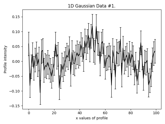
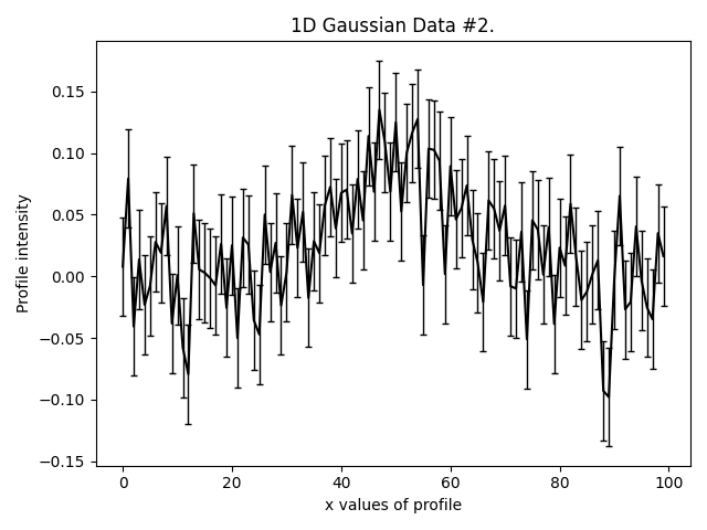

They are much lower signal-to-noise than the Gaussian’s in other examples. Graphical models extract a lot more information from lower quantity datasets, something we demonstrate explic in the HowToFit lectures on graphical models.
For each dataset we now create a corresponding Analysis class. By associating each dataset with an Analysis
class we are therefore associating it with a unique log_likelihood_function. If our dataset had many different
formats (e.g. images) it would be straight forward to write customized Analysis classes for each dataset.
analysis_list = []

for data, noise_map in zip(data_list, noise_map_list):

    analysis = Analysis(data=data, noise_map=noise_map)

    analysis_list.append(analysis)
We now compose the graphical model we will fit using the Model and Collection objects. We begin by setting up a
shared prior for their centre using a single GaussianPrior. This is passed to a unique Model for
each Gaussian and means that all three Gaussian’s are fitted wih the same value of centre. That is, we have
defined our graphical model to have a shared value of centre when it fits each dataset.
centre_shared_prior = af.GaussianPrior(mean=50.0, sigma=30.0)
We now set up three Model objects, each of which contain a Gaussian that is used to fit each of the
datasets we loaded above. Because all three of these Model’s use the centre_shared_prior the dimensionality of
parameter space is N=7, corresponding to three Gaussians with local parameters (normalization and sigma) and
a global parameter value of centre.
model_list = []

for model_index in range(len(data_list)):

    gaussian = af.Model(p.Gaussian)

    gaussian.centre = centre_shared_prior  # This prior is used by all 3 Gaussians!
    gaussian.normalization = af.LogUniformPrior(lower_limit=1e-6, upper_limit=1e6)
    gaussian.sigma = af.UniformPrior(lower_limit=0.0, upper_limit=25.0)

    model_list.append(gaussian)
To build our graphical model which fits multiple datasets, we simply pair each model-component to each Analysis
class, so that PyAutoFit knows that:
gaussian_0fitsdata_0viaanalysis_0.gaussian_1fitsdata_1viaanalysis_1.gaussian_2fitsdata_2viaanalysis_2.
The point where a Model and Analysis class meet is called a AnalysisFactor.
This term is used to denote that we are composing a ‘factor graph’. A factor defines a node on this graph where we have some data, a model, and we fit the two together. The ‘links’ between these different factors then define the global model we are fitting and the datasets used to fit it.
analysis_factor_list = []

for model, analysis in zip(model_list, analysis_list):

    analysis_factor = g.AnalysisFactor(prior_model=model, analysis=analysis)

    analysis_factor_list.append(analysis_factor)
We combine our AnalysisFactor’s into one, to compose the factor graph.
factor_graph = g.FactorGraphModel(*analysis_factor_list)
So, what does our factor graph looks like? Unfortunately, we haven’t yet build visualization of this into PyAutoFit, so you’ll have to make do with a description for now.
The factor graph above is made up of two components:
Nodes: these are points on the graph where we have a unique set of data and a model that is made up of a subset of
our overall graphical model. This is effectively the AnalysisFactor objects we created above.
Links: these define the model components and parameters that are shared across different nodes and thus retain the
same values when fitting different datasets.
We can now choose a non-linear search and fit the factor graph.
search = af.DynestyStatic()

result = search.fit(
    model=factor_graph.global_prior_model,
    analysis=factor_graph
)
This will fit the N=7 dimension parameter space where every Gaussian has a shared centre!
This is all expanded upon in the HowToFit chapter on graphical models, where we will give a more detailed description of why this approach to model-fitting extracts a lot more information than fitting each dataset one-by-one.
Expectation Propagation#
For large datasets, a graphical model may have hundreds, thousands, or hundreds of thousands of parameters. The high dimensionality of such a parameter space can make it inefficient or impossible to fit the model.
Fitting high dimensionality graphical models in PyAutoFit can use an Expectation Propagation (EP) framework to make scaling up feasible. This framework fits every dataset individually and pass messages throughout the graph to inform every fit the expected values of each parameter.
The following paper describes the EP framework in formal Bayesian notation:
Hierarchical Models#
A specific type of graphical model is a hierarchical model, where the shared parameter(s) of a graph are assumed to be drawn from a common parent distribution. Fitting these datasets simultanoeusly enables better estimate of this global distribution.
Hierarchical models can also be scaled up to large datasets via Expectation Propagation.