Multiple Datasets#
This cookbook illustrates how to fit multiple datasets simultaneously, where each dataset is fitted by a different
Analysis class.
The Analysis classes are combined to give an overall log likelihood function that is the sum of the
individual log likelihood functions, which a single model is fitted to via non-linear search.
If one has multiple observations of the same signal, it is often desirable to fit them simultaneously. This ensures that better constraints are placed on the model, as the full amount of information in the datasets is used.
In some scenarios, the signal may vary across the datasets in a way that requires that the model is updated accordingly. PyAutoFit provides tools to customize the model composition such that specific parameters of the model vary across the datasets.
This cookbook illustrates using observations of 3 1D Gaussians, which have the same centre (which is the same
for the model fitted to each dataset) but different normalization and sigma values (which vary for the model
fitted to each dataset).
It is common for each individual dataset to only constrain specific aspects of a model. The high level of model
customization provided by PyAutoFit ensures that composing a model that is appropriate for fitting large and diverse
datasets is straight forward. This is because different Analysis classes can be written for each dataset and combined.
Contents:
Model-Fit: Setup a model-fit to 3 datasets to illustrate multi-dataset fitting.
Analysis List: Create a list of
Analysisobjects, one for each dataset, which are fitted simultaneously.Analysis Factor: Wrap each
Analysisobject in anAnalysisFactor, which pairs it with the model and prepares it for model fitting.Factor Graph: Combine all
AnalysisFactorobjects into aFactorGraphModel, which represents a global model fit to multiple datasets.Result List: Use the output of fits to multiple datasets which are a list of
Resultobjects.Variable Model Across Datasets: Fit a model where certain parameters vary across the datasets whereas others stay fixed.
Relational Model: Fit models where certain parameters vary across the dataset as a user defined relation (e.g.
y = mx + c).Different Analysis Classes: Fit multiple datasets where each dataset is fitted by a different
Analysisclass, meaning that datasets with different formats can be fitted simultaneously.Interpolation: Fit multiple datasets with a model one-by-one and interpolation over a smoothly varying parameter (e.g. time) to infer the model between datasets.
Individual Sequential Searches: Fit multiple datasets where each dataset is fitted one-by-one sequentially.
Hierarchical / Graphical Models: Use hierarchical / graphical models to fit multiple datasets simultaneously, which fit for global trends in the model across the datasets.
Model Fit#
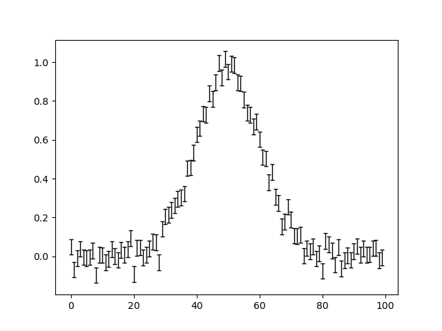
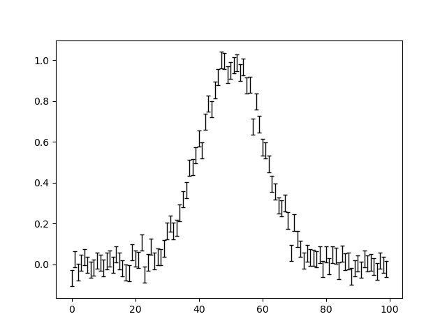
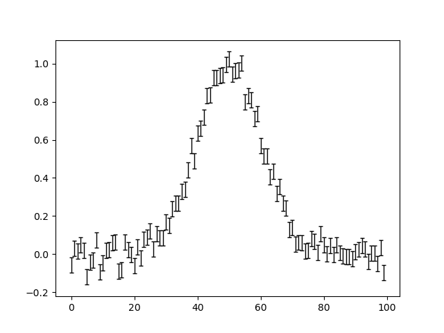
Load 3 1D Gaussian datasets from .json files in the directory autofit_workspace/dataset/.
All three datasets contain an identical signal, therefore fitting the same model to all three datasets simultaneously is appropriate.
Each dataset has a different noise realization, therefore fitting them simultaneously will offer improved constraints over individual fits.
dataset_size = 3

data_list = []
noise_map_list = []

for dataset_index in range(dataset_size):
    dataset_path = path.join(
        "dataset", "example_1d", f"gaussian_x1_identical_{dataset_index}"
    )

    data = af.util.numpy_array_from_json(file_path=path.join(dataset_path, "data.json"))
    data_list.append(data)

    noise_map = af.util.numpy_array_from_json(
        file_path=path.join(dataset_path, "noise_map.json")
    )
    noise_map_list.append(noise_map)
Plot all 3 datasets, including their error bars.
for data, noise_map in zip(data_list, noise_map_list):
    xvalues = range(data.shape[0])

    plt.errorbar(
        x=xvalues,
        y=data,
        yerr=noise_map,
        color="k",
        ecolor="k",
        linestyle=" ",
        elinewidth=1,
        capsize=2,
    )
    plt.show()
    plt.close()
Here is what the plots look like:
Create our model corresponding to a single 1D Gaussian that is fitted to all 3 datasets simultaneously.
model = af.Model(af.ex.Gaussian)

model.centre = af.UniformPrior(lower_limit=0.0, upper_limit=100.0)
model.normalization = af.LogUniformPrior(lower_limit=1e-2, upper_limit=1e2)
model.sigma = af.GaussianPrior(
    mean=10.0, sigma=5.0, lower_limit=0.0, upper_limit=np.inf
)
Analysis List#
Set up three instances of the Analysis class which fit 1D Gaussian.
analysis_list = []

for data, noise_map in zip(data_list, noise_map_list):

    analysis = af.ex.Analysis(data=data, noise_map=noise_map)
    analysis_list.append(analysis)
Analysis Factor#
Each analysis object is wrapped in an AnalysisFactor, which pairs it with the model and prepares it for use in a
factor graph. This step allows us to flexibly define how each dataset relates to the model.
The term “Factor” comes from factor graphs, a type of probabilistic graphical model. In this context, each factor represents the connection between one dataset and the shared model.
analysis_factor_list = []

for analysis in analysis_list:

    analysis_factor = af.AnalysisFactor(prior_model=model, analysis=analysis)

    analysis_factor_list.append(analysis_factor)
Factor Graph#
All AnalysisFactor objects are combined into a FactorGraphModel, which represents a global model fit to
multiple datasets using a graphical model structure.
The key outcomes of this setup are:
The individual log likelihoods from each
Analysisobject are summed to form the total log likelihood evaluated during the model-fitting process.Results from all datasets are output to a unified directory, with subdirectories for visualizations from each analysis object, as defined by their
visualizemethods.
This is a basic use of PyAutoFit’s graphical modeling capabilities, which support advanced hierarchical and probabilistic modeling for large, multi-dataset analyses.
factor_graph = af.FactorGraphModel(*analysis_factor_list)
To inspect the model, we print factor_graph.global_prior_model.info.
print(factor_graph.global_prior_model.info)
To fit multiple datasets, we pass the FactorGraphModel to a non-linear search.
Unlike single-dataset fitting, we now pass the factor_graph.global_prior_model as the model and
the factor_graph itself as the analysis object.
This structure enables simultaneous fitting of multiple datasets in a consistent and scalable way.
search = af.DynestyStatic(
    path_prefix="features", sample="rwalk", name="multiple_datasets_simple"
)

result_list = search.fit(model=factor_graph.global_prior_model, analysis=factor_graph)
Result List#
The result object returned by the fit is a list of the Result objects, which is described in the result cookbook.
Each Result in the list corresponds to each Analysis object in the analysis_list we passed to the fit.
The same model was fitted across all analyses, thus every Result in the result_list contains the same information
on the samples and the same max_log_likelihood_instance.
print(result_list[0].max_log_likelihood_instance.centre)
print(result_list[0].max_log_likelihood_instance.normalization)
print(result_list[0].max_log_likelihood_instance.sigma)

print(result_list[1].max_log_likelihood_instance.centre)
print(result_list[1].max_log_likelihood_instance.normalization)
print(result_list[1].max_log_likelihood_instance.sigma)
This gives the following output:
49.99110500540554
24.793778321608457
10.067848301502565
49.99110500540554
24.793778321608457
10.067848301502565
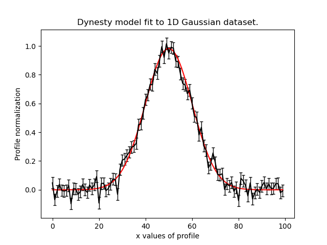
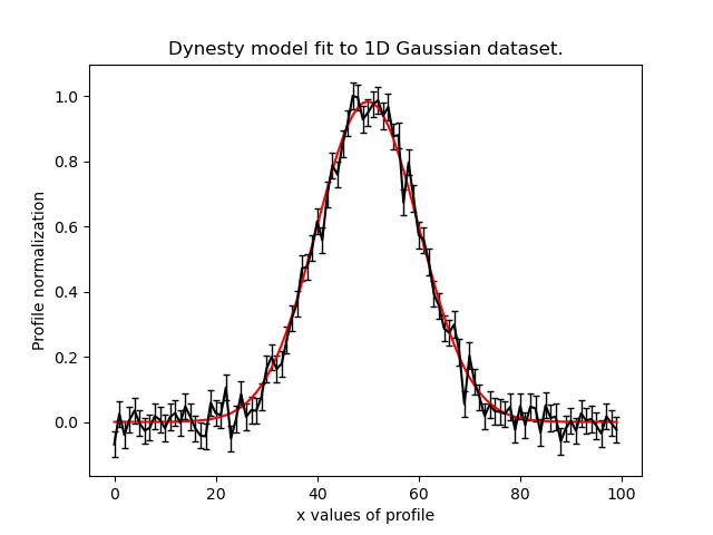
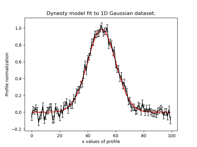
We can plot the model-fit to each dataset by iterating over the results:
for data, result in zip(data_list, result_list):
    instance = result.max_log_likelihood_instance

    model_data = instance.model_data_from(
        xvalues=np.arange(data.shape[0])
    )

    plt.errorbar(
        x=xvalues,
        y=data,
        yerr=noise_map,
        color="k",
        ecolor="k",
        elinewidth=1,
        capsize=2,
    )
    plt.plot(xvalues, model_data, color="r")
    plt.title("Dynesty model fit to 1D Gaussian dataset.")
    plt.xlabel("x values of profile")
    plt.ylabel("Profile normalization")
    plt.show()
    plt.close()
The image appears as follows:
Variable Model Across Datasets#
The same model was fitted to every dataset simultaneously because all 3 datasets contained an identical signal with only the noise varying across the datasets.
If the signal varied across the datasets, we would instead want to fit a different model to each dataset. The model
composition can be updated by changing the model passed to each AnalysisFactor.
We will use an example of 3 1D Gaussians which have the same centre but the normalization and sigma vary across
datasets:
dataset_path = path.join("dataset", "example_1d", "gaussian_x1_variable")

dataset_name_list = ["sigma_0", "sigma_1", "sigma_2"]

data_list = []
noise_map_list = []

for dataset_name in dataset_name_list:
    dataset_time_path = path.join(dataset_path, dataset_name)

    data = af.util.numpy_array_from_json(
        file_path=path.join(dataset_time_path, "data.json")
    )
    noise_map = af.util.numpy_array_from_json(
        file_path=path.join(dataset_time_path, "noise_map.json")
    )

    data_list.append(data)
    noise_map_list.append(noise_map)
Plotting these datasets shows that the normalization and`` sigma of each Gaussian vary.
for data, noise_map in zip(data_list, noise_map_list):
    xvalues = range(data.shape[0])

    af.ex.plot_profile_1d(xvalues=xvalues, profile_1d=data)
The images appear as follows:
The centre of all three 1D Gaussians are the same in each dataset, but their normalization and sigma values
are decreasing.
We will therefore fit a model to all three datasets simultaneously, whose centre is the same for all 3 datasets but
the normalization and sigma vary.
To do that, we use a summed list of Analysis objects, where each Analysis object contains a different dataset.
analysis_list = []

for data, noise_map in zip(data_list, noise_map_list):
    analysis = af.ex.Analysis(data=data, noise_map=noise_map)
    analysis_list.append(analysis)
We now update the model passed to each AnalysisFactor object to compose a model where:
The
centrevalues of the Gaussian fitted to every dataset in everyAnalysisobject are identical.The``normalization`` and
sigmavalue of the every Gaussian fitted to every dataset in everyAnalysisobject are different.
The model has 7 free parameters in total, x1 shared centre, x3 unique normalization’s and x3 unique sigma’s.
We do this by overwriting the normalization and sigma variables of the model passed to each AnalysisFactor object
with new priors, that make them free parameters of the model.
analysis_factor_list = []

for analysis in analysis_list:

    model_analysis = model.copy()

    model_analysis.normalization = af.LogUniformPrior(
        lower_limit=1e-2, upper_limit=1e2
    )
    model_analysis.sigma = af.GaussianPrior(
        mean=10.0, sigma=5.0, lower_limit=0.0, upper_limit=np.inf
    )

    analysis_factor = af.AnalysisFactor(prior_model=model_analysis, analysis=analysis)

    analysis_factor_list.append(analysis_factor)
To inspect this model, with extra parameters for each dataset created, we print factor_graph.global_prior_model.info.
factor_graph = af.FactorGraphModel(*analysis_factor_list)

print(factor_graph.global_prior_model.info)
This gives the following output:
Total Free Parameters = 7

model                                                                           GlobalPriorModel (N=7)
    0 - 2                                                                       Gaussian (N=3)

0 - 2
    centre                                                                      UniformPrior [3], lower_limit = 0.0, upper_limit = 100.0
0
    normalization                                                               LogUniformPrior [6], lower_limit = 0.01, upper_limit = 100.0
    sigma                                                                       GaussianPrior [7], mean = 10.0, sigma = 5.0
1
    normalization                                                               LogUniformPrior [8], lower_limit = 0.01, upper_limit = 100.0
    sigma                                                                       GaussianPrior [9], mean = 10.0, sigma = 5.0
2
    normalization                                                               LogUniformPrior [10], lower_limit = 0.01, upper_limit = 100.0
    sigma                                                                       GaussianPrior [11], mean = 10.0, sigma = 5.0
Fit this model to the data using dynesty.
search = af.DynestyStatic(
    path_prefix="features", sample="rwalk", name="multiple_datasets_free_sigma"
)

result_list = search.fit(model=factor_graph.global_prior_model, analysis=factor_graph)
The normalization and sigma values of the maximum log likelihood models fitted to each dataset are different,
which is shown by printing the sigma values of the maximum log likelihood instances of each result.
The centre values of the maximum log likelihood models fitted to each dataset are the same.
for result in result_list:
    instance = result.max_log_likelihood_instance

    print("Max Log Likelihood Model:")
    print("Centre = ", instance.centre)
    print("Normalization = ", instance.normalization)
    print("Sigma = ", instance.sigma)
    print()
This gives the following output:
Max Log Likelihood Model:
Centre =  50.06514422642149
Normalization =  50.25307503344711
Sigma =  10.021209148841097

Max Log Likelihood Model:
Centre =  50.06514422642149
Normalization =  50.21937758886209
Sigma =  20.143565300562734

Max Log Likelihood Model:
Centre =  50.06514422642149
Normalization =  50.35148002406068
Sigma =  30.49164712448904
Relational Model#
In the model above, two extra free parameters (normalization and ``sigma) were added for every dataset.
For just 3 datasets the model stays low dimensional and this is not a problem. However, for 30+ datasets the model will become complex and difficult to fit.
In these circumstances, one can instead compose a model where the parameters vary smoothly across the datasets via a user defined relation.
Below, we compose a model where the sigma value fitted to each dataset is computed according to:
``y = m * x + c`` : ``sigma`` = sigma_m * x + sigma_c``
Where x is an integer number specifying the index of the dataset (e.g. 1, 2 and 3).
By defining a relation of this form, sigma_m and sigma_c are the only free parameters of the model which vary
across the datasets.
Of more datasets are added the number of model parameters therefore does not increase.
model = af.Collection(gaussian=af.Model(af.ex.Gaussian))

sigma_m = af.UniformPrior(lower_limit=-10.0, upper_limit=10.0)
sigma_c = af.UniformPrior(lower_limit=-10.0, upper_limit=10.0)

x_list = [1.0, 2.0, 3.0]

analysis_factor_list = []

for x, analysis in zip(x_list, analysis_list):
    sigma_relation = (sigma_m * x) + sigma_c

    model_analysis = model.copy()
    model_analysis.gaussian.sigma = sigma_relation

    analysis_factor = af.AnalysisFactor(prior_model=model_analysis, analysis=analysis)

    analysis_factor_list.append(analysis_factor)
The factor graph is created and its info can be printed after the relational model has been defined.
factor_graph = af.FactorGraphModel(*analysis_factor_list)

print(factor_graph.global_prior_model.info)
This gives the following output:
Total Free Parameters = 4

model                                                                           GlobalPriorModel (N=4)
    0 - 2                                                                       Collection (N=4)
        gaussian                                                                Gaussian (N=4)
            sigma                                                               SumPrior (N=2)
                self                                                            MultiplePrior (N=1)

factor
    include_prior_factors                                                       True
0 - 2
    gaussian
        centre                                                                  UniformPrior [12], lower_limit = 0.0, upper_limit = 100.0
        normalization                                                           LogUniformPrior [13], lower_limit = 1e-06, upper_limit = 1000000.0
        sigma
            self
                sigma_m                                                         UniformPrior [15], lower_limit = -10.0, upper_limit = 10.0
            sigma_c                                                             UniformPrior [16], lower_limit = -10.0, upper_limit = 10.0
0
    gaussian
        sigma
            self
                x                                                               1.0
1
    gaussian
        sigma
            self
                x                                                               2.0
2
    gaussian
        sigma
            self
                x                                                               3.0
We can fit the model as per usual.
search = af.DynestyStatic(
    path_prefix="features", sample="rwalk", name="multiple_datasets_relation"
)

result_list = search.fit(model=factor_graph.global_prior_model, analysis=factor_graph)
The centre and sigma values of the maximum log likelihood models fitted to each dataset are different,
which is shown by printing the sigma values of the maximum log likelihood instances of each result.
They now follow the relation we defined above.
The centre normalization of the maximum log likelihood models fitted to each dataset are the same.
result_list = search.fit(model=model, analysis=analysis)

for result in result_list:
    instance = result.max_log_likelihood_instance

    print("Max Log Likelihood Model:")
    print("Centre = ", instance.centre)
    print("Normalization = ", instance.normalization)
    print("Sigma = ", instance.sigma)
    print()
This gives the following output:
Max Log Likelihood Model:
Centre =  50.04124738060383
Normalization =  50.330187946622246
Sigma =  10.04918613466697

Max Log Likelihood Model:
Centre =  50.04124738060383
Normalization =  50.330187946622246
Sigma =  20.04864425755685

Max Log Likelihood Model:
Centre =  50.04124738060383
Normalization =  50.330187946622246
Sigma =  30.048102380446732
Different Analysis Objects#
For simplicity, this example used a single Analysis class which fitted 1D Gaussian’s to 1D data.
For many problems one may have multiple datasets which are quite different in their format and structure. In this
situation, one can simply define unique Analysis objects for each type of dataset, which will contain a
unique log_likelihood_function and methods for visualization.
Hierarchical / Graphical Models#
The analysis factor API illustrated here can then be used to fit this large variety of datasets, noting that the the model can also be customized as necessary for fitting models to multiple datasets that are different in their format and structure.
This allows us to fit large heterogeneous datasets simultaneously, but also forms the basis of the graphical modeling API which can be used to fit complex models, such as hierarchical models, to extract more information from large datasets.
PyAutoFit has a dedicated feature set for fitting hierarchical and graphical models and interested readers should checkout the hierarchical and graphical modeling chapter of HowToFit (https://github.com/PyAutoLabs/HowToFit/blob/main/notebooks/chapter_3_graphical_models)
Interpolation#
One may have many datasets which vary according to a smooth function, for example a dataset taken over time where the signal varies smoothly as a function of time.
This could be fitted using the tools above, all at once. However, in many use cases this is not possible due to the model complexity, number of datasets or computational time.
An alternative approach is to fit each dataset individually, and then interpolate the results over the smoothly varying parameter (e.g. time) to estimate the model parameters at any point.
PyAutoFit has interpolation tools to do exactly this, which are described in the features/interpolation.ipynb
example.
Wrap Up#
We have shown how PyAutoFit can fit large datasets simultaneously, using custom models that vary specific parameters across the dataset.