Sensitivity Mapping#
Bayesian model comparison allows us to take a dataset, fit it with multiple models and use the Bayesian evidence to quantify which model objectively gives the best-fit following the principles of Occam’s Razor.
However, a complex model may not be favoured by model comparison not because it is the ‘wrong’ model, but simply because the dataset being fitted is not of a sufficient quality for the more complex model to be favoured. Sensitivity mapping addresses what quality of data would be needed for the more complex model to be favoured.
In order to do this, sensitivity mapping involves us writing a function that uses the model(s) to simulate a dataset. We then use this function to simulate many datasets, for many different models, and fit each dataset using the same model-fitting procedure we used to perform Bayesian model comparison. This allows us to infer how much of a Bayesian evidence increase we should expect for datasets of varying quality and / or models with different parameters.
Data#
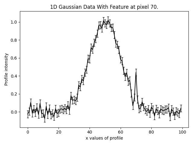
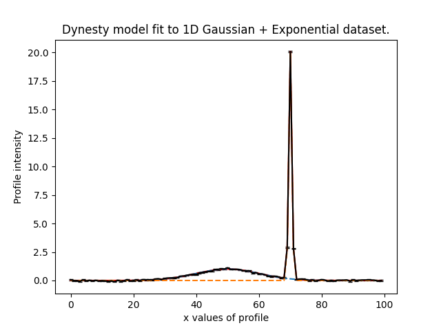
To illustrate sensitivity mapping we will again use the example of fitting 1D Gaussian’s in noisy data. This 1D data
includes a small feature to the right of the central Gaussian, a second Gaussian centred on pixel 70.
Model Comparison#
Before performing sensitivity mapping, we will quickly perform Bayesian model comparison on this data to get a sense
for whether the Gaussian feature is detectable and how much the Bayesian evidence increases when it is included in
the model.
We therefore fit the data using two models, one where the model is a single Gaussian.
model = af.Collection(gaussian_main=m.Gaussian)

search = af.DynestyStatic(
    path_prefix=path.join("features", "sensitivity_mapping", "single_gaussian"),
    nlive=100,
    iterations_per_full_update=500,
)

result_single = search.fit(model=model, analysis=analysis)
For the second model it contains two Gaussians. To avoid slow model-fitting and more clearly pronounce the results of
model comparison, we restrict the centre of the gaussian_feature to its true centre of 70 and sigma value of 0.5.
model = af.Collection(gaussian_main=m.Gaussian, gaussian_feature=m.Gaussian)
model.gaussian_feature.centre = 70.0
model.gaussian_feature.sigma = 0.5

search = af.DynestyStatic(
    path_prefix=path.join("features", "sensitivity_mapping", "two_gaussians"),
    nlive=100,
    iterations_per_full_update=500,
)

result_multiple = search.fit(model=model, analysis=analysis)
We can now print the log_evidence of each fit and confirm the model with two Gaussians was preferred to the model
with just one Gaussian.
print(result_single.samples.log_evidence)
print(result_multiple.samples.log_evidence)
On my laptop, the increase in Bayesian evidence for the more compelx model is ~30, which is significant.
The model comparison above shows that in this dataset, the Gaussian feature was detectable and that it increased the
Bayesian evidence by ~25. Furthermore, the normalization of this Gaussian was ~0.3.
A lower value of normalization makes the Gaussian fainter and harder to detect. We will demonstrate sensitivity mapping
by answering the following question, at what value of normalization does the Gaussian feature become undetectable and
not provide us with a noticeable increase in Bayesian evidence?
Base Model#
To begin, we define the base_model that we use to perform sensitivity mapping. This model is used to simulate every
dataset. It is also fitted to every simulated dataset without the extra model component below, to give us the Bayesian
evidence of the every simpler model to compare to the more complex model.
The base_model corresponds to the gaussian_main above.
base_model = af.Collection(gaussian_main=m.Gaussian)
Perturbation Model#
We now define the perturb_model, which is the model component whose parameters we iterate over to perform
sensitivity mapping. Many instances of the perturb_model are created and used to simulate the many datasets
that we fit. However, it is only included in half of the model-fits corresponding to the more complex models whose
Bayesian evidence we compare to the simpler model-fits consisting of just the base_model.
The perturb_model is therefore another Gaussian but now corresponds to the gaussian_feature above.
By fitting both of these models to every simulated dataset, we will therefore infer the Bayesian evidence of every
model to every dataset. Sensitivity mapping therefore maps out for what values of normalization in the gaussian_feature
does the more complex model-fit provide higher values of Bayesian evidence than the simpler model-fit. We also fix the
values ot the centre and sigma of the Gaussian so we only map over its normalization.
perturb_model = af.Model(m.Gaussian)
perturb_model.centre = 70.0
perturb_model.sigma = 0.5
perturb_model.normalization = af.UniformPrior(lower_limit=0.01, upper_limit=100.0)
Simulation#
We are performing sensitivity mapping to determine how bright the gaussian_feature needs to be in order to be
detectable. However, every simulated dataset must include the main_gaussian, as its presence in the data will effect
the detectability of the gaussian_feature.
We can pass the main_gaussian into the sensitivity mapping as the simulation_instance, meaning that it will be used
in the simulation of every dataset. For this example we use the inferred main_gaussian from one of the model-fits
performed above.
simulation_instance = result_single.instance
We now write the simulate_cls, which takes the instance of our model (defined above) and uses it to
simulate a dataset which is subsequently fitted.
Note that when this dataset is simulated, the quantity instance.perturb is used in the simulate_cls.
This is an instance of the gaussian_feature, and it is different every time the simulate_cls is called.
In this example, this instance.perturb corresponds to different gaussian_feature’s with values of
normalization ranging over 0.01 -> 100.0, such that our simulated datasets correspond to a very faint and very bright
gaussian features.
def __call__(instance, simulate_path):

    """
    Specify the number of pixels used to create the xvalues on which the 1D line of the profile is generated using and
    thus defining the number of data-points in our data.
    """
    pixels = 100
    xvalues = np.arange(pixels)

    """
    Evaluate the ``Gaussian`` and Exponential model instances at every xvalues to create their model profile and sum
    them together to create the overall model profile.

    This print statement will show that, when you run ``Sensitivity`` below the values of the perturbation use fixed
    values of ``centre=70`` and ``sigma=0.5``, whereas the normalization varies over the ``step_size`` based on its prior.
    """

    print(instance.perturb.centre)
    print(instance.perturb.normalization)
    print(instance.perturb.sigma)

    model_line = instance.gaussian_main.model_data_from(xvalues=xvalues) + instance.perturb.model_data_from(xvalues=xvalues)

    """Determine the noise (at a specified signal to noise level) in every pixel of our model profile."""
    signal_to_noise_ratio = 25.0
    noise = np.random.normal(0.0, 1.0 / signal_to_noise_ratio, pixels)

    """
    Add this noise to the model line to create the line data that is fitted, using the signal-to-noise ratio to compute
    noise-map of our data which is required when evaluating the chi-squared value of the likelihood.
    """
    data = model_line + noise
    noise_map = (1.0 / signal_to_noise_ratio) * np.ones(pixels)

    return Imaging(data=data, noise_map=noise_map)
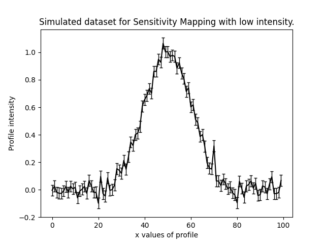
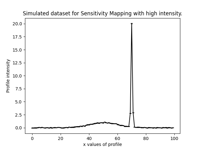
Here are what the two most extreme simulated datasets look like, corresponding to the highest and lowest normalization values
Summary#
We can now combine all of the objects created above and perform sensitivity mapping. The inputs to the Sensitivity
object below are:
simulation_instance: This is an instance of the model used to simulate every dataset that is fitted. In this example it contains an instance of thegaussian_mainmodel component.base_model: This is the simpler model that is fitted to every simulated dataset, which in this example is composed of a singleGaussiancalled thegaussian_main.perturb_model: This is the extra model component that alongside thebase_modelis fitted to every simulated dataset, which in this example is composed of twoGaussianscalled thegaussian_mainandgaussian_feature.simulate_cls: This is the function that uses theinstanceand many instances of theperturb_modelto simulate many datasets that are fitted with thebase_modelandbase_model+perturb_model.step_size: The size of steps over which the parameters in theperturb_modelare iterated. In this example, normalization has aLogUniformPriorwith lower limit 1e-4 and upper limit 1e2, therefore thestep_sizeof 0.5 will simulate and fit just 2 datasets where the normalization is 1e-4 and 1e2.number_of_cores: The number of cores over which the sensitivity mapping is performed, enabling parallel processing.
(Note that for brevity we have omitted a couple of extra inputs in this example, which can be found by going to the
full example script on the autofit_workspace).
sensitivity = s.Sensitivity(
    search=search,
    simulation_instance=simulation_instance,
    base_model=base_model,
    perturb_model=perturb_model,
    simulate_cls=simulate_cls,
    analysis_class=Analysis,
    step_size=0.5,
    number_of_cores=2,
)

sensitivity_result = sensitivity.run()
Here are what the fits to the two most extreme simulated datasets look like, for the models including the Gaussian feature.
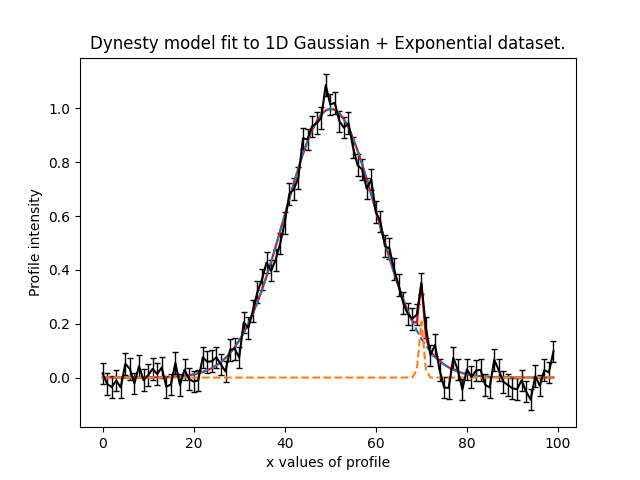
The key point to note is that for every dataset, we now have a model-fit with and without the model perturbation. By
compairing the Bayesian evidence of every pair of fits for every value of normalization we are able to determine when
our model was sensitivity to the Gaussian feature and therefore could detect it!