Search Chaining#
To perform a model-fit, we typically compose one model and fit it to our data using one non-linear search.
Search chaining fits many different models to a dataset using a chained sequence of non-linear searches. Initial fits are performed using simplified model parameterizations and faster non-linear fitting techniques. The results of these simplified fits can then be used to initialize fits using a higher dimensionality model with more detailed non-linear search.
To fit highly complex models our aim is therefore to granularize the fitting procedure into a series of bite-sized searches which are faster and more reliable than fitting the more complex model straight away.
Our ability to construct chained non-linear searches that perform model fitting more accurately and efficiently relies on our domain specific knowledge of the model fitting task. For example, we may know that our dataset contains multiple features that can be accurately fitted separately before performing a joint fit, or that certain parameters share minimal covariance such that allowing us to fix them to certain values in earlier model-fits.
We may also know tricks that can speed up the fitting of the initial model, for example reducing the size of the data or changing making a likelihood evaluation faster (most likely at the expense of the quality of the fit itself). By using chained searches speed-ups can be relaxed towards the end of the model-fitting sequence when we want the most precise, most accurate model that best fits the dataset available.
Data#
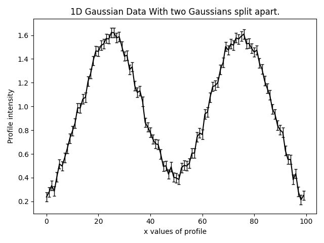
In this example we demonstrate search chaining using the example data where there are two Gaussians that are visibly
split:
Approach#
Instead of fitting them simultaneously using a single non-linear search consisting of N=6 parameters, we break this model-fit into a chained of three searches where:
The first model fits just the left
Gaussianwhere N=3.The second model fits just the right
Gaussianwhere again N=3.The final model is fitted with both
Gaussianswhere N=6. Crucially, the results of the first two searches are used to initialize the search and tell it the highest likelihood regions of parameter space.
By initially fitting parameter spaces of reduced complexity we can achieve a more efficient and reliable model-fitting procedure.
Search 1#
To fit the left Gaussian, our first analysis receive only half data removing the right Gaussian. Note that
this give a speed-up in log likelihood evaluation.
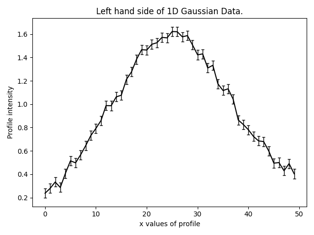
We first compose the model, which only represents the left hand Gaussian.
model_1 = af.Collection(gaussian_left=af.ex.Gaussian)
print(model_1.info)
The info attribute shows the model in a readable format.
This gives the following output:
gaussian_left
    centre                         UniformPrior, lower_limit = 0.0, upper_limit = 100.0
    normalization                  LogUniformPrior, lower_limit = 1e-06, upper_limit = 1000000.0
    sigma                          UniformPrior, lower_limit = 0.0, upper_limit = 25.0
We now create a search to fit this data. Given the simplicity of the model, we can use a low number of live points to achieve a fast model-fit (had we fitted the more complex model right away we could not of done this).
analysis_1 = af.ex.Analysis(data=data[0:50], noise_map=noise_map[0:50])

search_1 = af.DynestyStatic(
    name="search[1]__left_gaussian",
    path_prefix=path.join("features", "search_chaining"),
    nlive=30,
)

result_1 = search_1.fit(model=model_1, analysis=analysis_1)
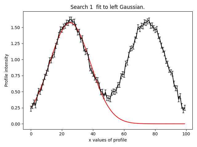
By plotting the result we can see we have fitted the left Gaussian reasonably well.
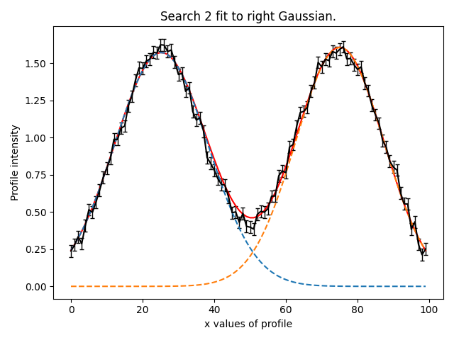
Search 2#
We now repeat the above process for the right Gaussian.
We could remove the data on the left like we did the Gaussian above. However, we are instead going to fit the full
dataset. To fit the left Gaussian we use the maximum log likelihood model of the model inferred in search 1.
For search chaining, PyAutoFit has many convenient methods for passing the results of a search to a subsequence
search. Below, we achieve this by passing the result of the search above as an instance.
model_2 = af.Collection(
    gaussian_left=result_1.instance.gaussian_left, gaussian_right=af.ex.Gaussian
)
The info attribute shows the model, including how parameters and priors were passed from result_1.
print(model_2.info)
This gives the following output:
gaussian_left
    centre                         25.43766022973362
    normalization                  51.98717889043411
    sigma                          12.99331932996352
gaussian_right
    centre                         UniformPrior, lower_limit = 0.0, upper_limit = 100.0
    normalization                  LogUniformPrior, lower_limit = 1e-06, upper_limit = 1000000.0
    sigma                          UniformPrior, lower_limit = 0.0, upper_limit = 25.0
We now run our second Dynesty search to fit the right Gaussian. We can again exploit the simplicity of the model
and use a low number of live points to achieve a fast model-fit.
analysis_2 = af.ex.Analysis(data=data, noise_map=noise_map)

search_2 = af.DynestyStatic(
    name="search[2]__right_gaussian",
    path_prefix=path.join("features", "search_chaining"),
    nlive=30,
)

result_2 = search_2.fit(model=model_2, analysis=analysis_2)
We can now see our model has successfully fitted both Gaussian’s:
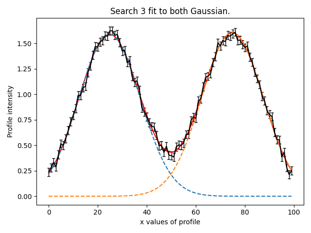
Search 3#
We now fit both Gaussians’s simultaneously, using the results of the previous two searches to initialize where
the non-linear searches parameter space.
To pass the result in this way we use the command result.model, which in contrast to result.instance above passes
the parameters not as the maximum log likelihood values but as GaussianPrior’s that are fitted for by the
non-linear search.
The mean and sigma value of each parmeter’s GaussianPrior are set using the results of searches 1 and
2 to ensure our model-fit only searches the high likelihood regions of parameter space.
model_3 = af.Collection(
    gaussian_left=result_1.model.gaussian_left,
    gaussian_right=result_2.model.gaussian_right,
)
The info attribute shows the model, including how parameters and priors were passed from result_1 and result_2.
print(model_3.info)
This gives the following output:
gaussian_left
    centre                         GaussianPrior, mean = 25.442897208320307, sigma = 20.0
    normalization                  GaussianPrior, mean = 51.98379634356712, sigma = 25.99189817178356
    sigma                          GaussianPrior, mean = 12.990448834848394, sigma = 6.495224417424197
gaussian_right
    centre                         GaussianPrior, mean = 75.052492251368, sigma = 20.0
    normalization                  GaussianPrior, mean = 48.757265879772476, sigma = 24.378632939886238
    sigma                          GaussianPrior, mean = 12.167662812557307, sigma = 6.083831406278653
analysis_3 = af.ex.Analysis(data=data, noise_map=noise_map)

search_3 = af.DynestyStatic(
    name="search[3]__both_gaussians",
    path_prefix=path.join("features", "search_chaining"),
    nlive=100,
)

result_3 = search_3.fit(model=model_3, analysis=analysis_3)
We can now see our model has successfully fitted both Gaussians simultaneously:
Wrap Up#
This fit used a technique called ‘prior passing’ to pass results from searches 1 and 2 to search 3. Full details of how
prior passing works can be found in the search_chaining.ipynb feature notebook.