Samples#
After a non-linear search has completed, it returns a Result object that contains information on fit, such as
the maximum likelihood model instance, the errors on each parameter and the Bayesian evidence.
This cookbook provides an overview of using the results.
Contents:
Model Fit: Perform a simple model-fit to create a
Samplesobject.Samples: The
Samplesobject contained in theResult, containing all non-linear samples (e.g. parameters, log likelihoods, etc.).Parameters: Accessing the parameters of the model from the samples.
Figures Of Merit: The log likelihood, log prior, log posterior and weight of every accepted sample.
Instances: Returning instances of the model corresponding to a particular sample (e.g. the maximum log likelihood).
Posterior / PDF: The median PDF model instance and PDF vectors of all model parameters via 1D marginalization.
Errors: The errors on every parameter estimated from the PDF, computed via marginalized 1D PDFs at an input sigma.
Samples Summary: A summary of the samples of the non-linear search (e.g. the maximum log likelihood model) which can be faster to load than the full set of samples.
Sample Instance: The model instance of any accepted sample.
Search Plots: Plots of the non-linear search, for example a corner plot or 1D PDF of every parameter.
Maximum Likelihood: The maximum log likelihood model value.
Bayesian Evidence: The log evidence estimated via a nested sampling algorithm.
Collection: Results created from models defined via a
Collectionobject.Lists: Extracting results as Python lists instead of instances.
Latex: Producing latex tables of results (e.g. for a paper).
The following sections outline how to use advanced features of the results, which you may skip on a first read:
Derived Quantities: Computing quantities and errors for quantities and parameters not included directly in the model.
Result Extension: Extend the
Resultobject with new attributes and methods (e.g.max_log_likelihood_model_data).Samples Filtering: Filter the
Samplesobject to only contain samples fulfilling certain criteria.
Model Fit#
To get a Samples object, we need to perform a model-fit, which you should be familiar after using a non-linear search.
result = search.fit(model=model, analysis=analysis)
Samples#
The result contains a Samples object, which contains all samples of the non-linear search.
Each sample corresponds to a set of model parameters that were evaluated and accepted by the non linear search, in this example emcee.
This includes their log likelihoods, which are used for computing additional information about the model-fit, for example the error on every parameter.
Our model-fit used the MCMC algorithm Emcee, so the Samples object returned is a SamplesMCMC object.
samples = result.samples

print("MCMC Samples: \n")
print(samples)
Parameters#
The parameters are stored as a list of lists, where:
The outer list is the size of the total number of samples.
The inner list is the size of the number of free parameters in the fit.
samples = result.samples

print("Sample 5's second parameter value (Gaussian -> normalization):")
print(samples.parameter_lists[4][1])
print("Sample 10's third parameter value (Gaussian -> sigma)")
print(samples.parameter_lists[9][2], "\n")
The output appears as follows:
Sample 5's second parameter value (Gaussian -> normalization):
1.561170345314133
Sample 10`s third parameter value (Gaussian -> sigma)
12.617071617003607
Figures Of Merit#
The Samples class contains the log likelihood, log prior, log posterior and weight_list of every accepted sample, where:
The
log_likelihoodis the value evaluated in thelog_likelihood_function.The
log_priorencodes information on how parameter priors map log likelihood values to log posterior values.The
log_posteriorislog_likelihood + log_prior.The
weightgives information on how samples are combined to estimate the posterior, which depends on type of search used (forEmceethey are all 1’s meaning they are weighted equally).
Lets inspect the last 10 values of each for the analysis.
print("log(likelihood), log(prior), log(posterior) and weight of the tenth sample.")
print(samples.log_likelihood_list[9])
print(samples.log_prior_list[9])
print(samples.log_posterior_list[9])
print(samples.weight_list[9])
The output appears as follows:
log(likelihood), log(prior), log(posterior) and weight of the tenth sample.
-5056.579275235516
0.743571372185727
-5055.83570386333
1.0
Instances#
Using the Samples object many results can be returned as an instance of the model, using the Python class structure
of the model composition.
For example, we can return the model parameters corresponding to the maximum log likelihood sample.
instance = samples.max_log_likelihood()

print("Max Log Likelihood Gaussian Instance:")
print("Centre = ", instance.centre)
print("Normalization = ", instance.normalization)
print("Sigma = ", instance.sigma, "\n")
The output appears as follows:
Max Log Likelihood `Gaussian` Instance:
Centre =  49.891590184286855
Normalization =  24.8187423966329
Sigma =  9.844319034011903
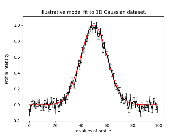
This makes it straight forward to plot the median PDF model:
model_data = instance.model_data_from(xvalues=np.arange(data.shape[0]))

plt.plot(range(data.shape[0]), data)
plt.plot(range(data.shape[0]), model_data)
plt.title("Illustrative model fit to 1D Gaussian profile data.")
plt.xlabel("x values of profile")
plt.ylabel("Profile normalization")
plt.show()
plt.close()
This plot appears as follows:
Posterior / PDF#
The result contains the full posterior information of our non-linear search, which can be used for parameter estimation.
The median pdf vector is available, which estimates every parameter via 1D marginalization of their PDFs.
instance = samples.median_pdf()

print("Median PDF Gaussian Instance:")
print("Centre = ", instance.centre)
print("Normalization = ", instance.normalization)
print("Sigma = ", instance.sigma, "\n")
The output appears as follows:
Median PDF `Gaussian` Instance:
Centre =  49.88646575581081
Normalization =  24.786319329440854
Sigma =  9.845578558662783
Errors#
Methods for computing error estimates on all parameters are provided.
This again uses 1D marginalization, now at an input sigma confidence limit.
instance_upper_sigma = samples.errors_at_upper_sigma(sigma=3.0)
instance_lower_sigma = samples.errors_at_lower_sigma(sigma=3.0)

print("Upper Error values (at 3.0 sigma confidence):")
print("Centre = ", instance_upper_sigma.centre)
print("Normalization = ", instance_upper_sigma.normalization)
print("Sigma = ", instance_upper_sigma.sigma, "\n")

print("lower Error values (at 3.0 sigma confidence):")
print("Centre = ", instance_lower_sigma.centre)
print("Normalization = ", instance_lower_sigma.normalization)
print("Sigma = ", instance_lower_sigma.sigma, "\n")
The output appears as follows:
Upper Error values (at 3.0 sigma confidence):
Centre =  0.34351559431248546
Normalization =  0.8210523662181224
Sigma =  0.36460084790041236

lower Error values (at 3.0 sigma confidence):
Centre =  0.36573975189415364
Normalization =  0.8277555014351385
Sigma =  0.318978781734252
They can also be returned at the values of the parameters at their error values.
instance_upper_values = samples.values_at_upper_sigma(sigma=3.0)
instance_lower_values = samples.values_at_lower_sigma(sigma=3.0)

print("Upper Parameter values w/ error (at 3.0 sigma confidence):")
print("Centre = ", instance_upper_values.centre)
print("Normalization = ", instance_upper_values.normalization)
print("Sigma = ", instance_upper_values.sigma, "\n")

print("lower Parameter values w/ errors (at 3.0 sigma confidence):")
print("Centre = ", instance_lower_values.centre)
print("Normalization = ", instance_lower_values.normalization)
print("Sigma = ", instance_lower_values.sigma, "\n")
The output appears as follows:
Upper Parameter values w/ error (at 3.0 sigma confidence):
Centre =  50.229981350123296
Normalization =  25.607371695658976
Sigma =  10.210179406563196

lower Parameter values w/ errors (at 3.0 sigma confidence):
Centre =  49.52072600391666
Normalization =  23.958563828005715
Sigma =  9.526599776928531
Samples Summary#
The samples summary contains a subset of results access via the Samples, for example the maximum likelihood model
and parameter error estimates.
Using the samples method above can be slow, as the quantities have to be computed from all non-linear search samples (e.g. computing errors requires that all samples are marginalized over). This information is stored directly in the samples summary and can therefore be accessed instantly.
print(samples.summary().max_log_likelihood_sample)
Sample Instance#
A non-linear search retains every model that is accepted during the model-fit.
We can create an instance of any model – below we create an instance of the last accepted model.
instance = samples.from_sample_index(sample_index=-1)

print("Gaussian Instance of last sample")
print("Centre = ", instance.centre)
print("Normalization = ", instance.normalization)
print("Sigma = ", instance.sigma, "\n")
The output appears as follows:
Gaussian Instance of last sample
Centre =  49.81486592598193
Normalization =  25.342058160043972
Sigma =  10.001029545296722
Search Plots#
The Probability Density Functions (PDF’s) of the results can be plotted using the Emcee’s visualization
tool corner.py, which is wrapped via the EmceePlotter object.
plotter = aplt.MCMCPlotter(samples=result.samples)
plotter.corner()
This plot appears as follows:

Maximum Likelihood#
The maximum log likelihood value of the model-fit can be estimated by simple taking the maximum of all log likelihoods of the samples.
If different models are fitted to the same dataset, this value can be compared to determine which model provides the best fit (e.g. which model has the highest maximum likelihood)?
print("Maximum Log Likelihood: \n")
print(max(samples.log_likelihood_list))
Bayesian Evidence#
If a nested sampling non-linear search is used, the evidence of the model is also available which enables Bayesian model comparison to be performed (given we are using Emcee, which is not a nested sampling algorithm, the log evidence is None).:
log_evidence = samples.log_evidence
print(f"Log Evidence: {log_evidence}")
The output appears as follows:
Log Evidence: None
Collection#
The examples correspond to a model where af.Model(Gaussian) was used to compose the model.
Below, we illustrate how the results API slightly changes if we compose our model using a Collection:
model = af.Collection(gaussian=af.ex.Gaussian, exponential=af.ex.Exponential)

analysis = af.ex.Analysis(data=data, noise_map=noise_map)

search = af.Emcee(
    nwalkers=50,
    nsteps=1000,
    number_of_cores=1,
)

result = search.fit(model=model, analysis=analysis)
The result.info shows the result for the model with both a Gaussian and Exponential profile.
print(result.info)
The output appears as follows:
Maximum Log Likelihood              -46.19567314
Maximum Log Posterior               999953.27251548

model                               Collection (N=6)
    gaussian                        Gaussian (N=3)
    exponential                     Exponential (N=3)

Maximum Log Likelihood Model:

gaussian
    centre                          49.914
    normalization                   24.635
    sigma                           9.851
exponential
    centre                          35.911
    normalization                   0.010
    rate                            5.219


Summary (3.0 sigma limits):

gaussian
    centre                          49.84 (44.87, 53.10)
    normalization                   24.67 (17.87, 38.81)
    sigma                           9.82 (6.93, 12.98)
exponential
    centre                          45.03 (1.03, 98.31)
    normalization                   0.00 (0.00, 0.67)
    rate                            4.88 (0.07, 9.91)


Summary (1.0 sigma limits):

gaussian
    centre                          49.84 (49.76, 49.93)
    normalization                   24.67 (24.46, 24.86)
    sigma                           9.82 (9.74, 9.90)
exponential
    centre                          45.03 (36.88, 54.81)
    normalization                   0.00 (0.00, 0.00)
    rate                            4.88 (3.73, 5.68)
Result instances again use the Python classes used to compose the model.
However, because our fit uses a Collection the instance has attribues named according to the names given to the
Collection, which above were gaussian and exponential.
For complex models, with a large number of model components and parameters, this offers a readable API to interpret the results.
instance = samples.max_log_likelihood()

print("Max Log Likelihood Gaussian Instance:")
print("Centre = ", instance.gaussian.centre)
print("Normalization = ", instance.gaussian.normalization)
print("Sigma = ", instance.gaussian.sigma, "\n")

print("Max Log Likelihood Exponential Instance:")
print("Centre = ", instance.exponential.centre)
print("Normalization = ", instance.exponential.normalization)
print("Sigma = ", instance.exponential.rate, "\n")
The output appears as follows:
Max Log Likelihood `Gaussian` Instance:
Centre =  49.91396277773068
Normalization =  24.63471453899279
Sigma =  9.850878941872832

Max Log Likelihood Exponential Instance:
Centre =  35.911326828717904
Normalization =  0.010107001861903789
Sigma =  5.2192591581876036
Lists#
All results can alternatively be returned as a 1D list of values, by passing as_instance=False:
max_lh_list = samples.max_log_likelihood(as_instance=False)
print("Max Log Likelihood Model Parameters: \n")
print(max_lh_list, "\n\n")
The output appears as follows:
Max Log Likelihood Model Parameters:

[49.91396277773068, 24.63471453899279, 9.850878941872832, 35.911326828717904, 0.010107001861903789, 5.2192591581876036]
The list above does not tell us which values correspond to which parameters.
The following quantities are available in the Model, where the order of their entries correspond to the parameters
in the ml_vector above:
paths: a list of tuples which give the path of every parameter in theModel.parameter_names: a list of shorthand parameter names derived from thepaths.parameter_labels: a list of parameter labels used when visualizing non-linear search results (see below).
For simple models like the one fitted in this tutorial, the quantities below are somewhat redundant. For the more complex models they are important for tracking the parameters of the model.
model = samples.model

print(model.paths)
print(model.parameter_names)
print(model.parameter_labels)
print(model.model_component_and_parameter_names)
print("\n")
The output appears as follows:
[('gaussian', 'centre'), ('gaussian', 'normalization'), ('gaussian', 'sigma'), ('exponential', 'centre'), ('exponential', 'normalization'), ('exponential', 'rate')]
['centre', 'normalization', 'sigma', 'centre', 'normalization', 'rate']
['x', 'norm', '\\sigma', 'x', 'norm', '\\lambda']
['gaussian_centre', 'gaussian_normalization', 'gaussian_sigma', 'exponential_centre', 'exponential_normalization', 'exponential_rate']
All the methods above are available as lists.
instance = samples.median_pdf(as_instance=False)
values_at_upper_sigma = samples.values_at_upper_sigma(sigma=3.0, as_instance=False)
values_at_lower_sigma = samples.values_at_lower_sigma(sigma=3.0, as_instance=False)
errors_at_upper_sigma = samples.errors_at_upper_sigma(sigma=3.0, as_instance=False)
errors_at_lower_sigma = samples.errors_at_lower_sigma(sigma=3.0, as_instance=False)
Latex#
If you are writing modeling results up in a paper, you can use inbuilt latex tools to create latex table code which you can copy to your .tex document.
By combining this with the filtering tools below, specific parameters can be included or removed from the latex.
Remember that the superscripts of a parameter are loaded from the config file notation/label.yaml, providing high
levels of customization for how the parameter names appear in the latex table. This is especially useful if your model
uses the same model components with the same parameter, which therefore need to be distinguished via superscripts.
latex = af.text.Samples.latex(
    samples=result.samples,
    median_pdf_model=True,
    sigma=3.0,
    name_to_label=True,
    include_name=True,
    include_quickmath=True,
    prefix="Example Prefix ",
    suffix=" \\[-2pt]",
)

print(latex)
The output appears as follows:
Example Prefix $x^{\rm{g}} = 49.88^{+0.37}_{-0.35}$ & $norm^{\rm{g}} = 24.83^{+0.82}_{-0.76}$ & $\sigma^{\rm{g}} = 9.84^{+0.35}_{-0.40}$ \[-2pt]
Derived Quantities (Advanced)#
The parameters centre, normalization and sigma are the model parameters of the Gaussian. They are sampled
directly by the non-linear search and we can therefore use the Samples object to easily determine their values and
errors.
Derived quantities (also called latent variables) are those which are not sampled directly by the non-linear search, but one may still wish to know their values and errors after the fit is complete. For example, what if we want the error on the full width half maximum (FWHM) of the Gaussian?
This is achieved by declaring a Latent class (subclass of af.Latent) on the Analysis class, whose
variables are computed after the non-linear search has completed. The analysis cookbook illustrates how to do this.
The example analysis used above declares a Latent (LatentExample) that computes the FWHM of the Gaussian
profile.
This leads to a number of noteworthy outputs:
A
latent.resultsfile is output to the results folder, which includes the value and error of all derived quantities based on the non-linear search samples (in this example only thefwhm).A
latent/samples.csvis output which lists every accepted sample’s value of every derived quantity, which is again analogous to thesamples.csvfile (in this example only thefwhm).A
latent/samples_summary.jsonis output which acts analogously tosamples_summary.jsonbut for the derived quantities of the model (in this example only thefwhm).
Derived quantities are also accessible via the Samples object, following a similar API to the model parameters:
latent = analysis.compute_latent_samples(result.samples)

instance = latent.max_log_likelihood()

print(f"Max Likelihood FWHM: {instance.gaussian.fwhm}")

instance = latent.median_pdf()

print(f"Median PDF FWHM {instance.gaussian.fwhm}")
Derived Errors (Advanced)#
Computing the errors of a quantity like the sigma of the Gaussian is simple, because it is sampled by the non-linear
search. Thus, to get their errors above we used the Samples object to simply marginalize over all over parameters
via the 1D Probability Density Function (PDF).
Computing errors on derived quantities is more tricky, because they are not sampled directly by the non-linear search. For example, what if we want the error on the full width half maximum (FWHM) of the Gaussian? In order to do this we need to create the PDF of that derived quantity, which we can then marginalize over using the same function we use to marginalize model parameters.
Below, we compute the FWHM of every accepted model sampled by the non-linear search and use this determine the PDF
of the FWHM. When combining the FWHM’s we weight each value by its weight. For Emcee, an MCMC algorithm, the
weight of every sample is 1, but weights may take different values for other non-linear searches.
In order to pass these samples to the function marginalize, which marginalizes over the PDF of the FWHM to compute
its error, we also pass the weight list of the samples.
(Computing the error on the FWHM could be done in much simpler ways than creating its PDF from the list of every sample. We chose this example for simplicity, in order to show this functionality, which can easily be extended to more complicated derived quantities.)
fwhm_list = []

for sample in samples.sample_list:
    instance = sample.instance_for_model(model=samples.model)

    sigma = instance.sigma

    fwhm = 2 * np.sqrt(2 * np.log(2)) * sigma

    fwhm_list.append(fwhm)

median_fwhm, lower_fwhm, upper_fwhm = af.marginalize(
    parameter_list=fwhm_list, sigma=3.0, weight_list=samples.weight_list
)

print(f"FWHM = {median_fwhm} ({upper_fwhm} {lower_fwhm}")
The output appears as follows:
FWHM = 23.065988076921947 (10.249510919377173 54.67455139997644
Samples Filtering (Advanced)#
Our samples object has the results for all three parameters in our model. However, we might only be interested in the results of a specific parameter.
The basic form of filtering specifies parameters via their path, which was printed above via the model and is printed again below.
samples = result.samples

print("Parameter paths in the model which are used for filtering:")
print(samples.model.paths)

print("All parameters of the very first sample")
print(samples.parameter_lists[0])

samples = samples.with_paths([("gaussian", "centre")])

print("All parameters of the very first sample (containing only the Gaussian centre.")
print(samples.parameter_lists[0])

print("Maximum Log Likelihood Model Instances (containing only the Gaussian centre):\n")
print(samples.max_log_likelihood(as_instance=False))
The output appears as follows:
Parameter paths in the model which are used for filtering:
[('gaussian', 'centre'), ('gaussian', 'normalization'), ('gaussian', 'sigma'), ('exponential', 'centre'), ('exponential', 'normalization'), ('exponential', 'rate')]

All parameters of the very first sample
[49.63779704398534, 1.1898799260824928, 12.68275074146554, 50.67597072491201, 0.7836791226321858, 5.07432721731388]

All parameters of the very first sample (containing only the Gaussian centre.
[49.63779704398534]

Maximum Log Likelihood Model Instances (containing only the Gaussian centre):
[49.880800628266506]
Above, we specified each path as a list of tuples of strings.
This is how the source code internally stores the path to different components of the model, but it is not in-profile_1d with the PyAutoFIT API used to compose a model.
We can alternatively use the following API:
samples = result.samples

samples = samples.with_paths(["gaussian.centre"])

print("All parameters of the very first sample (containing only the Gaussian centre).")
print(samples.parameter_lists[0])
The output appears as follows:
All parameters of the very first sample (containing only the Gaussian centre).
[49.63779704398534]
Above, we filtered the Samples but asking for all parameters which included the path (“gaussian”, “centre”).
We can alternatively filter the Samples object by removing all parameters with a certain path. Below, we remove
the Gaussian’s centre to be left with 2 parameters; the normalization and sigma.
samples = result.samples

print("Parameter paths in the model which are used for filtering:")
print(samples.model.paths)

print("All parameters of the very first sample")
print(samples.parameter_lists[0])

samples = samples.without_paths(["gaussian.centre"])

print(
    "All parameters of the very first sample (containing only the Gaussian normalization and sigma)."
)
print(samples.parameter_lists[0])
The output appears as follows:
Parameter paths in the model which are used for filtering:
[('gaussian', 'centre'), ('gaussian', 'normalization'), ('gaussian', 'sigma'), ('exponential', 'centre'), ('exponential', 'normalization'), ('exponential', 'rate')]
All parameters of the very first sample
[49.63779704398534, 1.1898799260824928, 12.68275074146554, 50.67597072491201, 0.7836791226321858, 5.07432721731388]
All parameters of the very first sample (containing only the Gaussian normalization and sigma).
[1.1898799260824928, 12.68275074146554, 50.67597072491201, 0.7836791226321858, 5.07432721731388]