PyAutoFit

PyAutoFit is a Python based probabilistic programming language for model fitting and Bayesian inference of large datasets.

The basic PyAutoFit API allows us a user to quickly compose a probabilistic model and fit it to data via a log likelihood function, using a range of non-linear search algorithms (e.g. MCMC, nested sampling).

Users can then set up PyAutoFit scientific workflow, which enables streamlined modeling of small datasets with tools to scale up to large datasets.

PyAutoFit supports advanced statistical methods, most notably a big data framework for Bayesian hierarchical analysis.

Getting Started

The following links are useful for new starters:

• The PyAutoFit readthedocs, which includes an installation guide and an overview of PyAutoFit’s core features.

• The introduction Jupyter Notebook on Binder, where you can try PyAutoFit in a web browser (without installation).

• The autofit_workspace GitHub repository, which includes example scripts and the HowToFit Jupyter notebook lectures which give new users a step-by-step introduction to PyAutoFit.

Support

Support for installation issues, help with Fit modeling and using PyAutoFit is available by raising an issue on the GitHub issues page.

We also offer support on the PyAutoFit Slack channel, where we also provide the latest updates on PyAutoFit. Slack is invitation-only, so if you’d like to join send an email requesting an invite.

HowToFit

For users less familiar with Bayesian inference and scientific analysis you may wish to read through the HowToFits lectures. These teach you the basic principles of Bayesian inference, with the content pitched at undergraduate level and above.

A complete overview of the lectures is provided on the HowToFit readthedocs page

API Overview

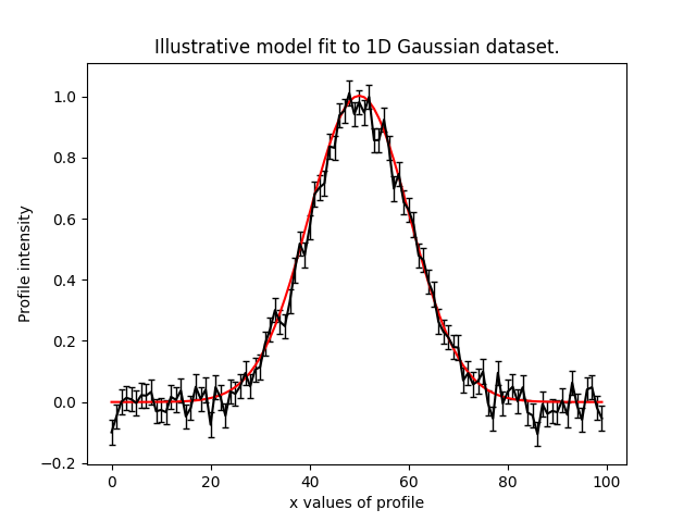
To illustrate the PyAutoFit API, we use an illustrative toy model of fitting a one-dimensional Gaussian to noisy 1D data. Here’s the data (black) and the model (red) we’ll fit:

We define our model, a 1D Gaussian by writing a Python class using the format below:

class Gaussian:

    def __init__(
        self,
        centre=0.0,        # <- PyAutoFit recognises these
        normalization=0.1, # <- constructor arguments are
        sigma=0.01,        # <- the Gaussian's parameters.
    ):
        self.centre = centre
        self.normalization = normalization
        self.sigma = sigma

    """
    An instance of the Gaussian class will be available during model fitting.

    This method will be used to fit the model to data and compute a likelihood.
    """

    def model_data_1d_via_xvalues_from(self, xvalues):

        transformed_xvalues = xvalues - self.centre

        return (self.normalization / (self.sigma * (2.0 * np.pi) ** 0.5)) * \
                np.exp(-0.5 * (transformed_xvalues / self.sigma) ** 2.0)

PyAutoFit recognises that this Gaussian may be treated as a model component whose parameters can be fitted for via a non-linear search like emcee.

To fit this Gaussian to the data we create an Analysis object, which gives PyAutoFit the data and a log_likelihood_function describing how to fit the data with the model:

class Analysis(af.Analysis):

    def __init__(self, data, noise_map):

        self.data = data
        self.noise_map = noise_map

    def log_likelihood_function(self, instance):

        """
        The 'instance' that comes into this method is an instance of the Gaussian class
        above, with the parameters set to values chosen by the non-linear search.
        """

        print("Gaussian Instance:")
        print("Centre = ", instance.centre)
        print("normalization = ", instance.normalization)
        print("Sigma = ", instance.sigma)

        """
        We fit the ``data`` with the Gaussian instance, using its
        "model_data_1d_via_xvalues_from" function to create the model data.
        """

        xvalues = np.arange(self.data.shape[0])

        model_data = instance.model_data_1d_via_xvalues_from(xvalues=xvalues)
        residual_map = self.data - model_data
        chi_squared_map = (residual_map / self.noise_map) ** 2.0
        log_likelihood = -0.5 * sum(chi_squared_map)

        return log_likelihood

We can now fit our model to the data using a non-linear search:

model = af.Model(Gaussian)

analysis = Analysis(data=data, noise_map=noise_map)

emcee = af.Emcee(nwalkers=50, nsteps=2000)

result = emcee.fit(model=model, analysis=analysis)

The result contains information on the model-fit, for example the parameter samples, maximum log likelihood model and marginalized probability density functions.